R package authors sometimes like to add the letter “r” to package names (for example, the tidyverse packages). baRcodeR also has an extra “r” at the end as well. I thought I could use some available data see if the letter frequency changes compared to the English language average.
I used two data sets. The first is the percentage frequency of letters in the English language taken from this table of English letter frequencies at the Cornell Math Explorers Club. I originally used the first table from [this wikipedia page] (https://en.wikipedia.org/wiki/Letter_frequency) except that the percentages seem to sum to 108. A text file of the table is available here.
The second dataset is a file of R package names. While it is possible to query CRAN to get the information, Gergely Daróczi has already done so. The csv file can be download here.
avg_distribution <- read.delim("../../static/files/mec_letter_frequency.txt", stringsAsFactors = F)
rpackage_info <- read.csv("../../static/files/results.csv", stringsAsFactors = F)
avg_distribution <- read.delim("mec_letter_frequency.txt", stringsAsFactors = F)
rpackage_info <- read.csv("results.csv", stringsAsFactors = F)The avg_distribution table contains the count and frequency (in percentage) of each letter in descending order.
names(avg_distribution) <- c("Letter", "avg_count", "avg_frequency")The rpackage_info data frame contains a great deal of useful information including the date of first release and the number of version.
head(rpackage_info)## name first_release versions archived index
## 1 BN <NA> 0 TRUE 1
## 2 DP <NA> 0 TRUE 2
## 3 Rm <NA> 0 TRUE 3
## 4 a <NA> 0 TRUE 4
## 5 pn <NA> 0 TRUE 5
## 6 ratetables 1997-10-08 17:56:00 1 TRUE 6To get frequencies, we need to split each letter in the package names, and then make a summary table for each letter summing the number of occurrences.
Splitting each letter apart can be done with the strsplit function.
split_letters <- unlist(strsplit(rpackage_info$name, split = ""))
head(split_letters)
## [1] "B" "N" "D" "P" "R" "m"However, we do have a mix of upper and lowercase letters. Those can be converted with the tolower function.
split_letters <- tolower(split_letters)
head(split_letters)
## [1] "b" "n" "d" "p" "r" "m"We can peek in at the unique characters.
unique(split_letters)## [1] "b" "n" "d" "p" "r" "m" "a" "t" "e" "l" "s" "o" "z" "c" "k" "y" "i" "f" "u"
## [20] "g" "q" "h" "v" "x" "w" "5" "1" "0" "7" "4" "j" "." "2" "3" "9" "8" "6"And now we can make a table summarizing the counts of each letter.
char_frequencies <- as.data.frame(table(split_letters))
char_frequencies
## split_letters Freq
## 1 . 490
## 2 0 81
## 3 1 78
## 4 2 282
## 5 3 77
## 6 4 79
## 7 5 22
## 8 6 20
## 9 7 15
## 10 8 10
## 11 9 16
## 12 a 8301
## 13 b 2258
## 14 c 5206
## 15 d 3837
## 16 e 9339
## 17 f 1877
## 18 g 3165
## 19 h 1848
## 20 i 6633
## 21 j 249
## 22 k 1044
## 23 l 5195
## 24 m 5419
## 25 n 4865
## 26 o 6257
## 27 p 4955
## 28 q 480
## 29 r 8790
## 30 s 8266
## 31 t 7524
## 32 u 2263
## 33 v 1380
## 34 w 897
## 35 x 830
## 36 y 1229
## 37 z 305We only want to look at alphabetical characters so we will drop all the other characters. Then we can convert the raw count into a percentage to compare with our average frequency.
char_frequencies <- char_frequencies[char_frequencies$split_letters %in% letters,]
char_frequencies$Freq <- char_frequencies$Freq * 100/sum(char_frequencies$Freq)
char_frequencies
## split_letters Freq
## 12 a 8.1054954
## 13 b 2.2048197
## 14 c 5.0833887
## 15 d 3.7466313
## 16 e 9.1190485
## 17 f 1.8327930
## 18 g 3.0904581
## 19 h 1.8044760
## 20 i 6.4767801
## 21 j 0.2431356
## 22 k 1.0194118
## 23 l 5.0726477
## 24 m 5.2913721
## 25 n 4.7504199
## 26 o 6.1096356
## 27 p 4.8383002
## 28 q 0.4686951
## 29 r 8.5829786
## 30 s 8.0713198
## 31 t 7.3467953
## 32 u 2.2097020
## 33 v 1.3474983
## 34 w 0.8758739
## 35 x 0.8104519
## 36 y 1.2000547
## 37 z 0.2978167ggplot2 can be used to visualize the scatterplot.
avg_distribution$Letter <- tolower(avg_distribution$Letter)
char_frequencies<- dplyr::left_join(char_frequencies, avg_distribution, by = c("split_letters" = "Letter"))
## Warning: Column `split_letters`/`Letter` joining factor and character vector,
## coercing into character vectorlibrary(ggplot2)
ggplot(char_frequencies, aes(x = avg_frequency, y = Freq)) +
geom_point() +
geom_abline(slope = 1) +
theme_classic() +
geom_text(aes(label = split_letters), nudge_x = 0.2) +
labs(x="Average Percentage in English Language", y = "Percentage in R Package Names")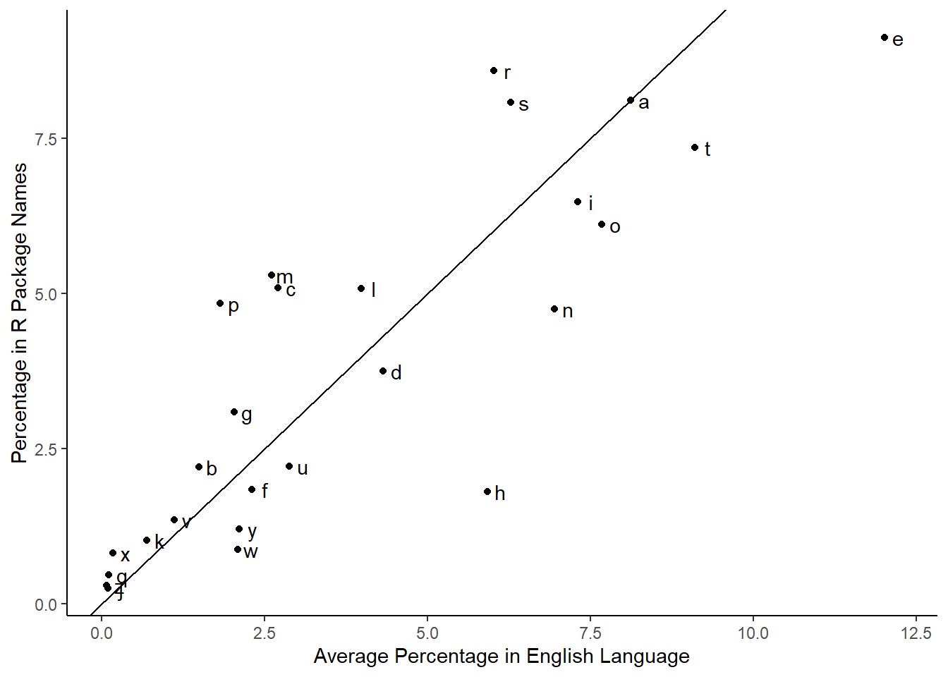
Letters above the line increased in frequency in R package names compared to the average while letters below the line decreased in frequency.
The order of most to least common in the English language is etaoinsrhdlucmfywgpbvkxqjz.
Based on the R package name letter frequencies, the order is erastiomclpndgubfhvykwxqzj.
So “r” moves from the eighth most common letter to the second most common letter.
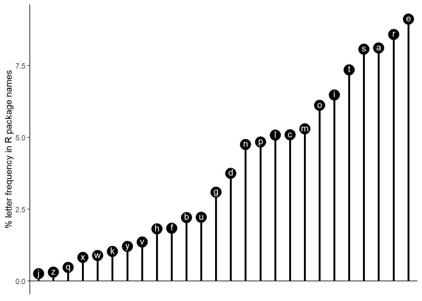
We can represent the frequency as a lollipop chart.
char_frequencies <- char_frequencies[order(char_frequencies$Freq, decreasing = T),]
char_frequencies$split_letters <- factor(char_frequencies$split_letters, levels = rev(char_frequencies$split_letters))

ggplot(char_frequencies, aes(x=split_letters, y = Freq)) +
  geom_point(size = 6) +
  geom_segment(aes(x=split_letters, y = 0, xend = split_letters, yend = Freq), size = 1.1) +
  theme_classic() +
  geom_hline(yintercept = 0) +
  geom_text(aes(label = split_letters), colour = "white", nudge_y = 0.05) +
  labs(y = "% letter frequency in R package names") +
  # coord_flip() +
  theme(axis.line.x = element_blank(), axis.text.x = element_blank(), axis.ticks.x = element_blank(), axis.title.x = element_blank())
While the above chart shows percent frequency of letters, it doesn’t show how much the frequencies differ from the average frequency for each letter.
We can modify the data to calculate percent differences, or rather how much the percent change is.
char_frequencies$pct_difference <- (char_frequencies$Freq - char_frequencies$avg_frequency) * 100 / char_frequencies$avg_frequency
char_frequencies$split_letters <- as.character(char_frequencies$split_letters)
char_frequencies <- char_frequencies[order(char_frequencies$pct_difference, decreasing = T),]
char_frequencies$split_letters <- factor(char_frequencies$split_letters, levels = rev(char_frequencies$split_letters))

head(char_frequencies)
## split_letters Freq avg_count avg_frequency pct_difference
## 24 x 0.8104519 315 0.17 376.7364
## 17 q 0.4686951 205 0.11 326.0864
## 26 z 0.2978167 128 0.07 325.4524
## 16 p 4.8383002 3316 1.82 165.8407
## 10 j 0.2431356 188 0.10 143.1356
## 13 m 5.2913721 4761 2.61 102.7346ggplot(char_frequencies, aes(x=split_letters, y = pct_difference)) +
geom_point(size = 6) +
geom_segment(aes(x=split_letters, y = 0, xend = split_letters, yend = pct_difference), size = 1.1) +
theme_classic() +
geom_hline(yintercept=0) +
geom_text(aes(label = split_letters), colour = "white", nudge_x = 0.13) +
labs(y = "% change in letter frequency from \n R package names to English language average") +
coord_flip() +
theme(axis.line.y = element_blank(), axis.text.y = element_blank(), axis.ticks.y = element_blank(), axis.title.y = element_blank())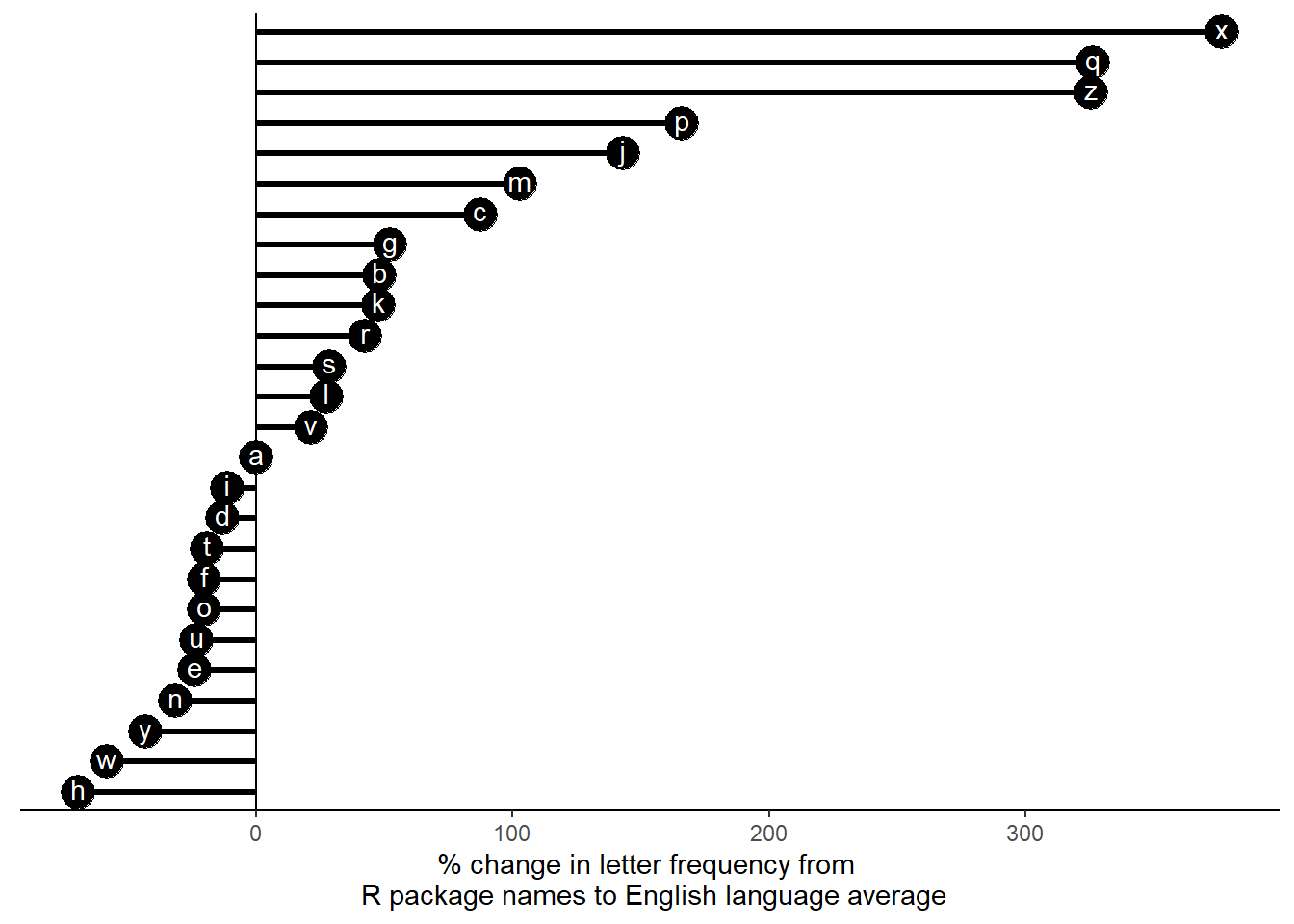
Many letters showed greater percent changes compared to the average letter frequency than the letter “r”. The rarer letters such as “x” and “z” show more than a 300 percent increase in frequency. Additionally, it is curious that all the vowels either showed almost no change or a decrease.
We can also track the changes in the proportion of a letter across years.
library(tidyverse)## Warning: package 'tidyverse' was built under R version 3.6.2## -- Attaching packages ----------------------------------------------------- tidyverse 1.3.0 --## v tibble 2.1.3 v dplyr 0.8.4
## v tidyr 1.0.2 v stringr 1.4.0
## v readr 1.3.1 v forcats 0.4.0
## v purrr 0.3.3## Warning: package 'tibble' was built under R version 3.6.2## Warning: package 'tidyr' was built under R version 3.6.2## Warning: package 'dplyr' was built under R version 3.6.2## -- Conflicts -------------------------------------------------------- tidyverse_conflicts() --
## x dplyr::filter() masks stats::filter()
## x dplyr::lag() masks stats::lag()count_single <- function(x, letter){
sum(tolower(unlist(strsplit(x, split=""))) == letter)
}
count_letters <- function(x){
sum(tolower(unlist(strsplit(x, split=""))) %in% letters)
}
year_pct <- rpackage_info %>% group_by(lubridate::year(first_release)) %>% summarise(count_name = count_letters(name), letter_count = count_single(name, "r")) %>% mutate(pct_freq = letter_count * 100 / count_name)
names(year_pct)[1] <- "year"
ggplot(year_pct, aes(x = year, y = pct_freq)) +
geom_point() +
geom_smooth(method="lm") +
theme_classic() + labs(x="Year", y = "Percent frequency of the letter r")## Warning: Removed 1 rows containing non-finite values (stat_smooth).## Warning: Removed 1 rows containing missing values (geom_point).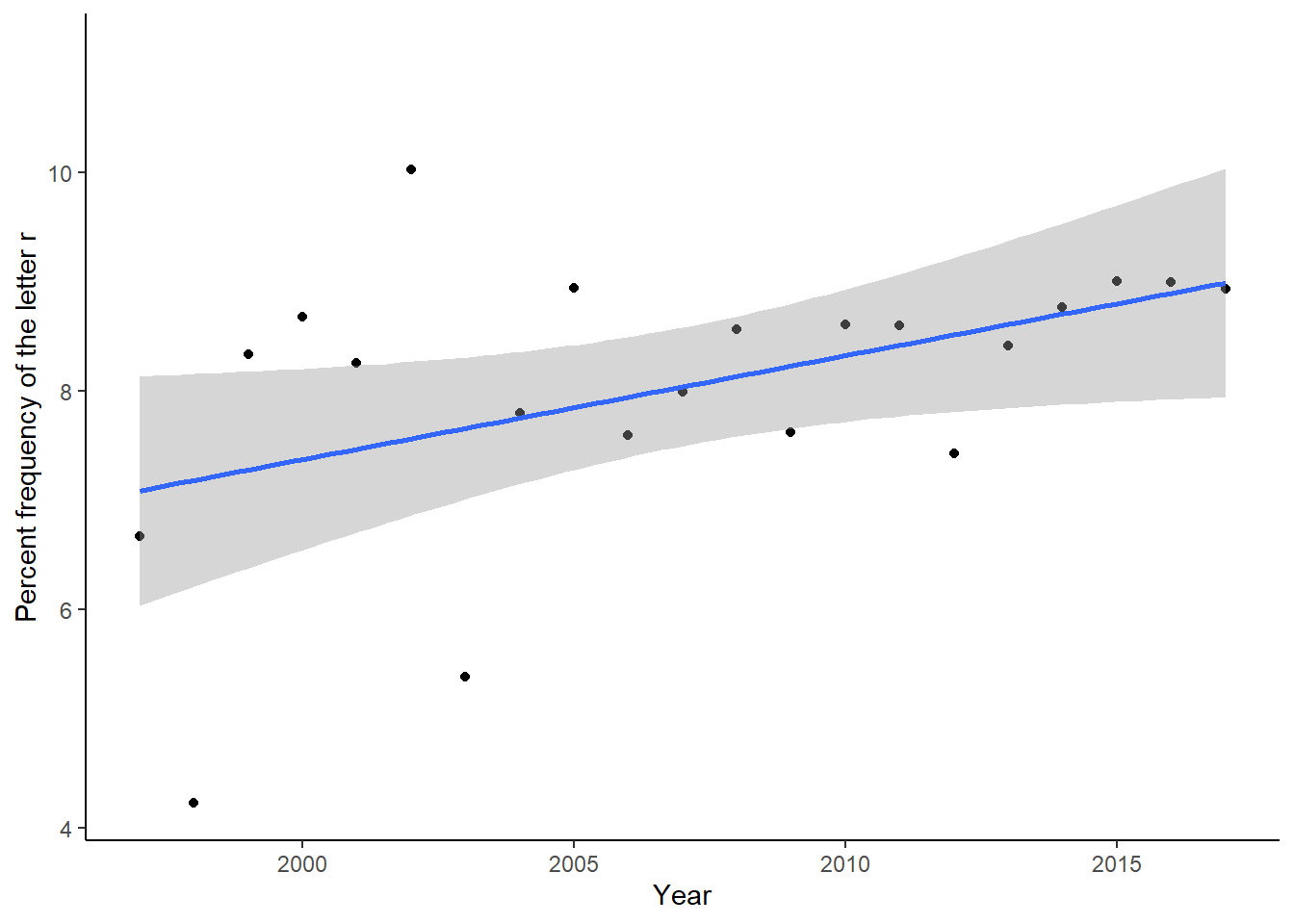
The letter “r” increases and jumps around in percentage frequency over the years.
year_pct <- rpackage_info %>% group_by(lubridate::year(first_release)) %>% summarise(count_name = count_letters(name), letter_count = count_single(name, "p")) %>% mutate(pct_freq = letter_count * 100 / count_name)

names(year_pct)[1] <- "year"

ggplot(year_pct, aes(x = year, y = pct_freq)) +
  geom_point() +
  geom_smooth(method="lm") +
  theme_classic() + labs(x="Year", y = "Percent frequency of the letter p")
## Warning: Removed 1 rows containing non-finite values (stat_smooth).## Warning: Removed 1 rows containing missing values (geom_point).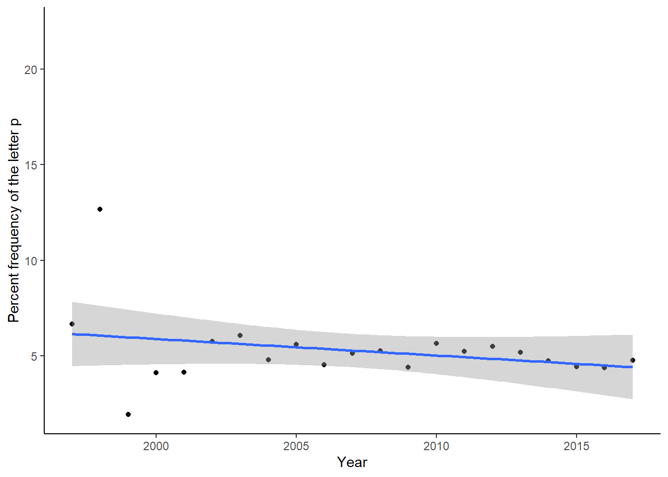
Others, like “p” remain relatively constant.
year_pct <- rpackage_info %>% group_by(lubridate::year(first_release)) %>% summarise(count_name = count_letters(name), letter_count = count_single(name, "s")) %>% mutate(pct_freq = letter_count * 100 / count_name)

names(year_pct)[1] <- "year"

ggplot(year_pct, aes(x = year, y = pct_freq)) +
  geom_point() +
  geom_smooth(method="lm") +
  theme_classic() + labs(x="Year", y = "Percent frequency of the letter s")
## Warning: Removed 1 rows containing non-finite values (stat_smooth).## Warning: Removed 1 rows containing missing values (geom_point).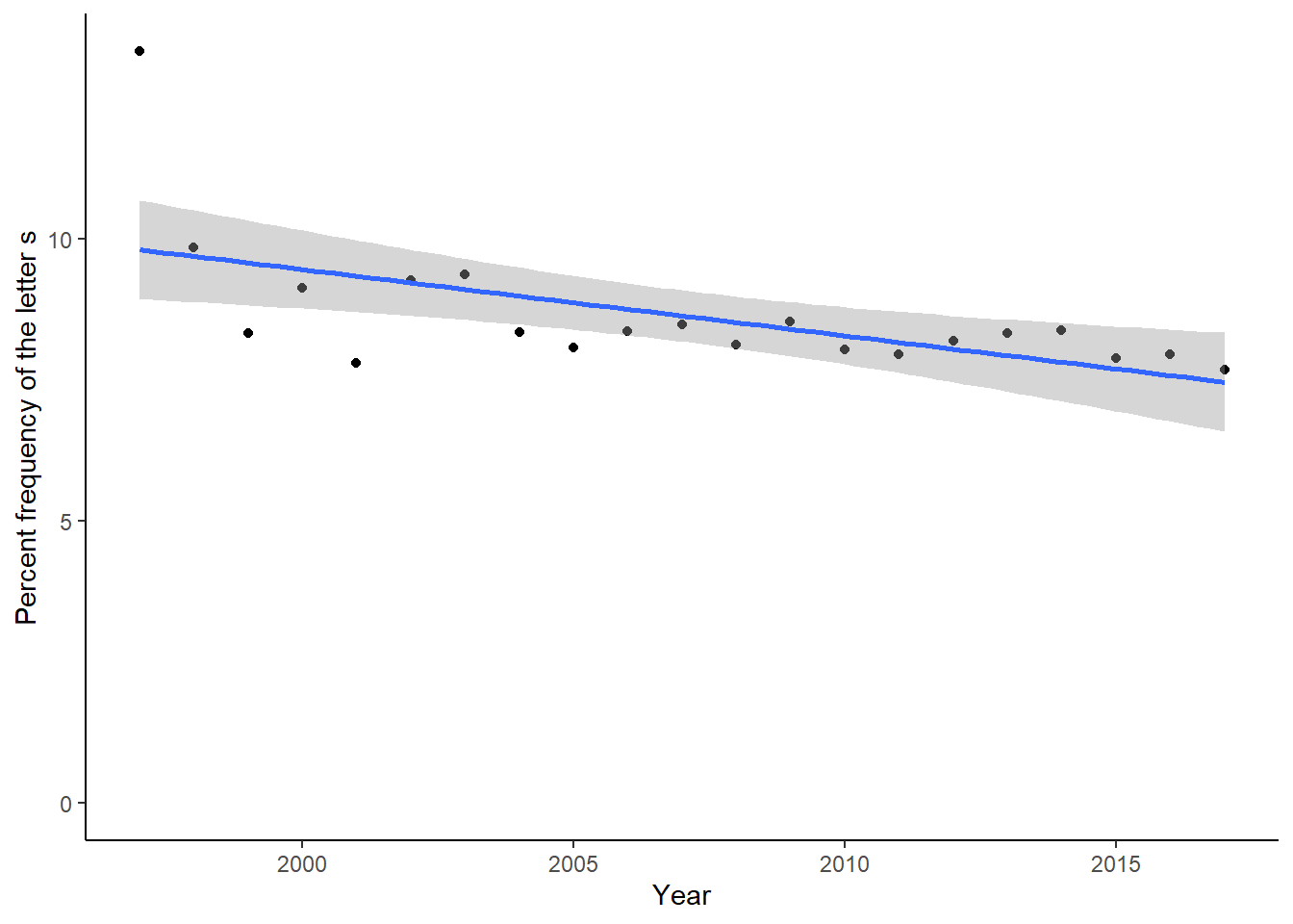
And we have letters such as “s” have steadily popular in package names.
sessionInfo()## R version 3.6.1 (2019-07-05)
## Platform: x86_64-w64-mingw32/x64 (64-bit)
## Running under: Windows 10 x64 (build 18363)
##
## Matrix products: default
##
## locale:
## [1] LC_COLLATE=English_Canada.1252 LC_CTYPE=English_Canada.1252
## [3] LC_MONETARY=English_Canada.1252 LC_NUMERIC=C
## [5] LC_TIME=English_Canada.1252
##
## attached base packages:
## [1] stats graphics grDevices utils datasets methods base
##
## other attached packages:
## [1] forcats_0.4.0 stringr_1.4.0 dplyr_0.8.4 purrr_0.3.3
## [5] readr_1.3.1 tidyr_1.0.2 tibble_2.1.3 tidyverse_1.3.0
## [9] ggplot2_3.2.1
##
## loaded via a namespace (and not attached):
## [1] tidyselect_1.0.0 xfun_0.12 haven_2.2.0 lattice_0.20-38
## [5] colorspace_1.4-1 generics_0.0.2 vctrs_0.2.2 htmltools_0.4.0
## [9] yaml_2.2.1 rlang_0.4.4 pillar_1.4.3 glue_1.3.1
## [13] withr_2.1.2 DBI_1.1.0 dbplyr_1.4.2 modelr_0.1.5
## [17] readxl_1.3.1 lifecycle_0.1.0 munsell_0.5.0 blogdown_0.17
## [21] gtable_0.3.0 cellranger_1.1.0 rvest_0.3.5 evaluate_0.14
## [25] labeling_0.3 knitr_1.28 fansi_0.4.1 broom_0.5.4
## [29] Rcpp_1.0.3 scales_1.1.0 backports_1.1.5 jsonlite_1.6.1
## [33] farver_2.0.3 fs_1.3.1 hms_0.5.3 digest_0.6.23
## [37] stringi_1.4.3 bookdown_0.17 grid_3.6.1 cli_2.0.1
## [41] tools_3.6.1 magrittr_1.5 lazyeval_0.2.2 crayon_1.3.4
## [45] pkgconfig_2.0.3 xml2_1.2.2 reprex_0.3.0 lubridate_1.7.4
## [49] rstudioapi_0.10 assertthat_0.2.1 rmarkdown_2.1 httr_1.4.1
## [53] R6_2.4.1 nlme_3.1-144 compiler_3.6.1