From the last post, Vancouver has several common genus in its collection, such as Prunus and Acer. So rather than analyzing the diversity of Vancouver tree species on a species level, we could, with the help of some R packages, visualize the variety of taxonomic groups.
First, we format the Vancouver tree dataset similar to before to get the proper scientific name. This is the same formatting done in the previous post.
library(dplyr)
library(purrr)
library(tidyr)
# read in trees shp
# read in trees df
trees_df<-read.csv("StreetTrees_CityWide.csv", stringsAsFactors = F)
trees_df<-trees_df[trees_df$LATITUDE > 40 & trees_df$LONGITUDE < -100,]
trees_df$SCIENTIFIC_NAME <- paste(trees_df$GENUS_NAME, trees_df$SPECIES_NM)trees_df$GENUS_NAME <- as.character(trees_df$GENUS_NAME)
trees_df$SPECIES_NAME <- as.character(trees_df$SPECIES_NAME)
species_correction <- function(genus, species){
if(species == "SPECIES"){
return(genus)
} else if (length(grep("\\sX$", species)) > 0){
return(paste(genus," x ", unlist(strsplit(species, " "))[[1]]))
} else {
return(paste(genus, species))
}
}
trees_df$SCIENTIFIC_NAME <- map2_chr(trees_df$GENUS_NAME, trees_df$SPECIES_NAME, species_correction)
head(trees_df)## TREE_ID CIVIC_NUMBER STD_STREET NEIGHBOURHOOD_NAME ON_STREET
## 1 589 4694 W 8TH AV WEST POINT GREY BLANCA ST
## 2 592 1799 W KING EDWARD AV SHAUGHNESSY W KING EDWARD AV
## 3 594 2401 W 1ST AV KITSILANO W 1ST AV
## 5 596 2428 W 1ST AV KITSILANO W 1ST AV
## 6 598 2428 W 1ST AV KITSILANO W 1ST AV
## 7 599 1725 BALSAM ST KITSILANO W 1ST AV
## ON_STREET_BLOCK STREET_SIDE_NAME ASSIGNED HEIGHT_RANGE_ID DIAMETER
## 1 2400 EVEN N 5 32.0
## 2 1700 MED N 1 3.0
## 3 2400 ODD N 4 14.0
## 5 2400 EVEN N 2 11.0
## 6 2400 EVEN N 2 3.0
## 7 2400 EVEN N 2 13.5
## DATE_PLANTED PLANT_AREA ROOT_BARRIER CURB CULTIVAR_NAME GENUS_NAME
## 1 20180128 B N Y ALNUS
## 2 20100104 30 N Y ABIES
## 3 20180128 B N Y PINUS
## 5 20180128 B N Y PRUNUS
## 6 20180128 B N Y PRUNUS
## 7 20180128 B N Y PICEA
## SPECIES_NAME COMMON_NAME LATITUDE LONGITUDE SCIENTIFIC_NAME
## 1 RUGOSA SPECKLED ALDER 49.26532 -123.2150 ALNUS RUGOSA
## 2 GRANDIS GRAND FIR 49.24952 -123.1457 ABIES GRANDIS
## 3 NIGRA AUSTRIAN PINE 49.27096 -123.1599 PINUS NIGRA
## 5 SARGENTII SARGENT FLOWERING CHERRY 49.27083 -123.1602 PRUNUS SARGENTII
## 6 SARGENTII SARGENT FLOWERING CHERRY 49.27084 -123.1605 PRUNUS SARGENTII
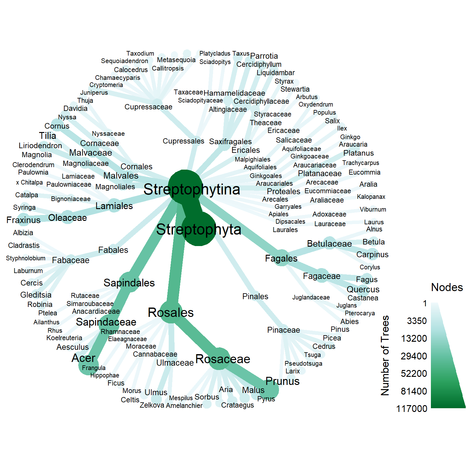
## 7 ABIES NORWAY SPRUCE 49.27083 -123.1600 PICEA ABIESTo get taxonomic information, we can take advantage of the rOpenSci package taxa. This package provides a function lookup_tax_data which will query NCBI taxonomy. We can then use the package metacoder to visualize a “heat tree” for datasets of taxon. This package was originally developed for next generation sequencing and metabarcoding in identifying species from DNA. So the “heat tree” has been diverted from its original purpose but still works very well.
# install.packages("taxa", "metacoder")
library(taxa)
library(metacoder)
## This is metacoder verison 0.3.3 (stable)To save on space, we will make a table containing each species in our Vancouver dataset and the number of times it occurs.
species_df <- as.data.frame(table(trees_df$SCIENTIFIC_NAME))
names(species_df)<- c("SCIENTIFIC_NAME", "count")
head(species_df)
## SCIENTIFIC_NAME count
## 1 ABIES 33
## 2 ABIES BALSAMEA 7
## 3 ABIES CONCOLOR 7
## 4 ABIES FRASERI 1
## 5 ABIES GRANDIS 65
## 6 ABIES NORDMANNIANA 1Querying the NCBI servers for information takes a long time depending on the number of request. If you sign up for a NCBI API key (instructions here), and add it to your .Renviron file which is usually located in your home directory.
We are going to use the taxize function classification to obtain the taxonomy of each species. Then, we are inserting the taxonomy for each species back into the trees_df so each tree has an associated taxonomy in column.
library(taxize)

species_classifications <- classification(species_df$SCIENTIFIC_NAME, db = "ncbi", rows = 1)
This creates a list of data frames containing the taxonomy. We can then extract the taxonomy information by iterating over the classification list and drop all species which do not have taxonomy.
class_to_df <- function(x, ranking){
  if(!is.na(x)){
  return(x$name[x$rank == ranking])
    }
}

# species_df <- species_df[species_df$SCIENTIFIC_NAME != "PINUS THUNBERGII", ]
species_df$superkingdom <- as.character(sapply(species_classifications, class_to_df, ranking="superkingdom"))
species_df$kingdom <- as.character(sapply(species_classifications, class_to_df, ranking="kingdom"))
species_df$phylum <- as.character(sapply(species_classifications, class_to_df, ranking="phylum"))
species_df$subphylum <- as.character(sapply(species_classifications, class_to_df, ranking="subphylum"))
species_df$subclass <- as.character(sapply(species_classifications, class_to_df, ranking="subclass"))
species_df$order <- as.character(sapply(species_classifications, class_to_df, ranking="order"))
species_df$family <- as.character(sapply(species_classifications, class_to_df, ranking="family"))
species_df$genus <- as.character(sapply(species_classifications, class_to_df, ranking="genus"))
species_df$species <- as.character(sapply(species_classifications, class_to_df, ranking="species"))

species_df <- species_df[species_df$superkingdom != "NULL", ]
We can then join the taxonomy back to the original data set so each tree has its own taxonomy. We also drop the other columns not related to the taxonomy.
trees_df_class <- left_join(trees_df, species_df)
kept_columns <- c('SCIENTIFIC_NAME', 'phylum', 'subphylum', 'order', 'family', 'genus', 'species')
trees_df_class <- trees_df_class[, kept_columns]
## write.csv(trees_df_class, "trees_taxa.csv", row.names=F)
Next, we use the parse_tax_data function to … … parse the taxonomy columns in the data frame into a tax_map object.
## Warning: package 'taxize' was built under R version 3.6.2By making a ranks vector, we tell parse_tax_data which columns contain the taxonomy and the ranking order.
ranks <- c('phylum', 'subphylum', 'order', 'family', 'genus', 'species')
obj <- parse_tax_data(trees_df_class, class_cols = ranks, named_by_rank = T)
## The following 7305 of 124349 (5.87%) input indexes have `NA` in their classifications:
## 29, 33, 37, 38, 64 ... 124296, 124328, 124329, 124342, 124347The resulting object returned from parse_tax_data is actually a special R6 object rather than the typical data.frame or S4 object. But since metacoder is based on using taxa, it can directly interface with the R6 object produced and we can produce a “heat tree” without any further manipulation.
set.seed(123)

tax_graph <- obj %>%
  filter_taxa(nchar(taxon_names)!=0) %>%
  filter_taxa(taxon_ranks == "genus", supertaxa = TRUE) %>%
  heat_tree(node_label = taxon_names,
            node_size = n_obs,
            node_label_size = n_obs,
            node_color = n_obs,
            node_size_range = c(0.01, .05),
            node_color_range = RColorBrewer::brewer.pal(5, "BuGn"),
            node_label_size_range = c(0.02, 0.05),
            node_color_axis_label = "Number of Trees")

tax_graph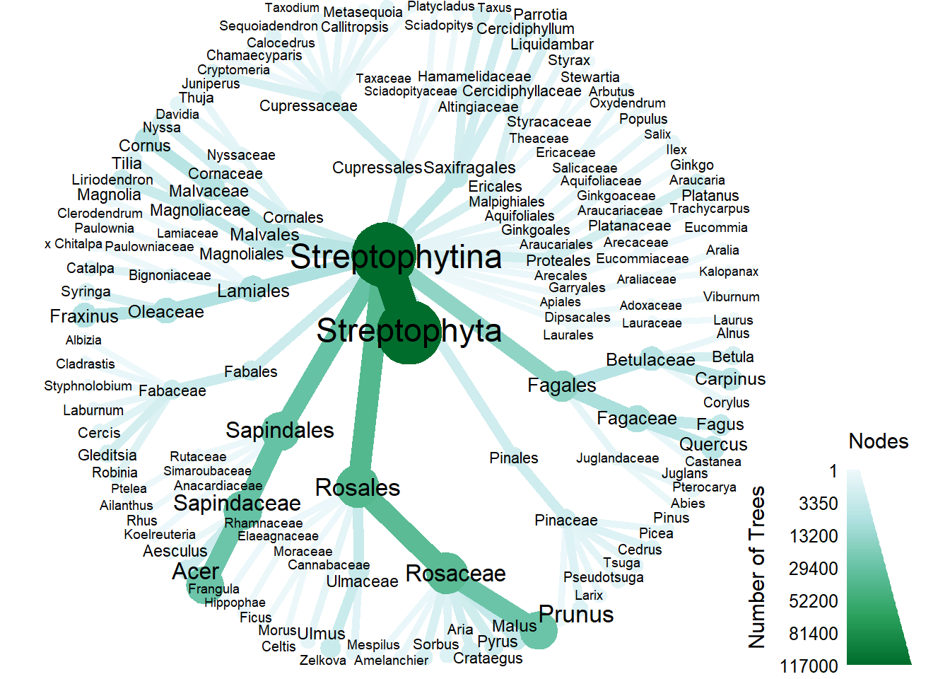
The tax_map is filtered to only the genus level in order to produce a legible visualization compared to a species level heat tree.
Node size is related to number of observations. The most common genus in Vancouver are Prunus and Acer.
sessionInfo()## R version 3.6.1 (2019-07-05)
## Platform: x86_64-w64-mingw32/x64 (64-bit)
## Running under: Windows 10 x64 (build 18363)
##
## Matrix products: default
##
## locale:
## [1] LC_COLLATE=English_Canada.1252 LC_CTYPE=English_Canada.1252
## [3] LC_MONETARY=English_Canada.1252 LC_NUMERIC=C
## [5] LC_TIME=English_Canada.1252
##
## attached base packages:
## [1] stats graphics grDevices utils datasets methods base
##
## other attached packages:
## [1] taxize_0.9.91 metacoder_0.3.3 taxa_0.3.2 tidyr_1.0.2
## [5] purrr_0.3.3 dplyr_0.8.4
##
## loaded via a namespace (and not attached):
## [1] zoo_1.8-7 tidyselect_1.0.0 xfun_0.12 reshape2_1.4.3
## [5] lattice_0.20-38 colorspace_1.4-1 vctrs_0.2.2 htmltools_0.4.0
## [9] viridisLite_0.3.0 yaml_2.2.1 rlang_0.4.4 pillar_1.4.3
## [13] httpcode_0.2.0 glue_1.3.1 RColorBrewer_1.1-2 foreach_1.4.7
## [17] lifecycle_0.1.0 plyr_1.8.5 stringr_1.4.0 ggfittext_0.8.1
## [21] munsell_0.5.0 blogdown_0.17 gtable_0.3.0 codetools_0.2-16
## [25] evaluate_0.14 labeling_0.3 knitr_1.28 parallel_3.6.1
## [29] curl_4.3 fansi_0.4.1 Rcpp_1.0.3 scales_1.1.0
## [33] jsonlite_1.6.1 farver_2.0.3 ggplot2_3.2.1 digest_0.6.23
## [37] stringi_1.4.3 bookdown_0.17 grid_3.6.1 cli_2.0.1
## [41] tools_3.6.1 magrittr_1.5 lazyeval_0.2.2 tibble_2.1.3
## [45] bold_0.9.0 crul_0.9.0 crayon_1.3.4 ape_5.3
## [49] pkgconfig_2.0.3 data.table_1.12.8 xml2_1.2.2 assertthat_0.2.1
## [53] rmarkdown_2.1 reshape_0.8.8 iterators_1.0.12 R6_2.4.1
## [57] igraph_1.2.4.2 nlme_3.1-144 compiler_3.6.1Notes:
The taxa package has a function lookup_tax_data which queries NCBI for and creates a tax_map object. However, I have problems using tree_df, possibly due to the large amount of associated data which has to go into the tax_map object. Additionally, the taxon_ranks are not created directly when using lookup_tax_data. The example code for using lookup_tax_data is below. Also weirdly, lookup_tax_data breaks when querying for Pinus thunbergii the last three times I tried.
trees_df <- trees_df[trees_df$SCIENTIFIC_NAME != "PINUS THUNBERGII", c("SCIENTIFIC_NAME", "GENUS_NAME")]
tax_env <- lookup_tax_data(trees_df, type = "taxon_name", column = "SCIENTIFIC_NAME", database = "ncbi")