Following from the past post, this post is focused on visualizing diversity through the package vegan and also maps showing the presence of native/introduced trees.
The most important code in this post is manipulating Spatial*DataFrames.
The same files will be read in, including the native/introduced status downloaded from USDA PLANTS.
library(rgdal)
library(sp)
library(raster)
library(dplyr)
library(httr)
library(rvest)
library(purrr)
library(tidyr)
# read in trees df
trees_df<-read.csv("StreetTrees_CityWide.csv", stringsAsFactors = F)
trees_df<-trees_df[trees_df$LATITUDE > 40 & trees_df$LONGITUDE < -100,]
# read in polygons
locmap<-readOGR("cov_localareas.kml", "local_areas_region", stringsAsFactors = F)## OGR data source with driver: KML
## Source: "C:\Users\YIHANWU\Documents\Stuff\blogdown-ywu\content\post\cov_localareas.kml", layer: "local_areas_region"
## with 22 features
## It has 2 fields# read in native/introduced
city_plant_info <- read.csv("vancouver_info.csv")
# extract tree data
trees_df$SCIENTIFIC_NAME <- paste(trees_df$GENUS_NAME, trees_df$SPECIES_NAME)trees_df$GENUS_NAME <- as.character(trees_df$GENUS_NAME)
trees_df$SPECIES_NM <- as.character(trees_df$SPECIES_NAME)
species_correction <- function(genus, species){
if(species == "SPECIES"){
return(genus)
} else if (length(grep("\\sX$", species)) > 0){
return(paste(genus," x ", unlist(strsplit(species, " "))[[1]]))
} else {
return(paste(genus, species))
}
}
trees_df$SCIENTIFIC_NAME <- map2_chr(trees_df$GENUS_NAME, trees_df$SPECIES_NAME, species_correction)
head(trees_df)## TREE_ID CIVIC_NUMBER STD_STREET NEIGHBOURHOOD_NAME ON_STREET
## 1 589 4694 W 8TH AV WEST POINT GREY BLANCA ST
## 2 592 1799 W KING EDWARD AV SHAUGHNESSY W KING EDWARD AV
## 3 594 2401 W 1ST AV KITSILANO W 1ST AV
## 5 596 2428 W 1ST AV KITSILANO W 1ST AV
## 6 598 2428 W 1ST AV KITSILANO W 1ST AV
## 7 599 1725 BALSAM ST KITSILANO W 1ST AV
## ON_STREET_BLOCK STREET_SIDE_NAME ASSIGNED HEIGHT_RANGE_ID DIAMETER
## 1 2400 EVEN N 5 32.0
## 2 1700 MED N 1 3.0
## 3 2400 ODD N 4 14.0
## 5 2400 EVEN N 2 11.0
## 6 2400 EVEN N 2 3.0
## 7 2400 EVEN N 2 13.5
## DATE_PLANTED PLANT_AREA ROOT_BARRIER CURB CULTIVAR_NAME GENUS_NAME
## 1 20180128 B N Y ALNUS
## 2 20100104 30 N Y ABIES
## 3 20180128 B N Y PINUS
## 5 20180128 B N Y PRUNUS
## 6 20180128 B N Y PRUNUS
## 7 20180128 B N Y PICEA
## SPECIES_NAME COMMON_NAME LATITUDE LONGITUDE SCIENTIFIC_NAME
## 1 RUGOSA SPECKLED ALDER 49.26532 -123.2150 ALNUS RUGOSA
## 2 GRANDIS GRAND FIR 49.24952 -123.1457 ABIES GRANDIS
## 3 NIGRA AUSTRIAN PINE 49.27096 -123.1599 PINUS NIGRA
## 5 SARGENTII SARGENT FLOWERING CHERRY 49.27083 -123.1602 PRUNUS SARGENTII
## 6 SARGENTII SARGENT FLOWERING CHERRY 49.27084 -123.1605 PRUNUS SARGENTII
## 7 ABIES NORWAY SPRUCE 49.27083 -123.1600 PICEA ABIES
## SPECIES_NM
## 1 RUGOSA
## 2 GRANDIS
## 3 NIGRA
## 5 SARGENTII
## 6 SARGENTII
## 7 ABIESWe can attach the native/introduced status through a dplyr::left_join.
trees_df <- left_join(trees_df, city_plant_info)## Joining, by = "SCIENTIFIC_NAME"## Warning: Column `SCIENTIFIC_NAME` joining character vector and factor, coercing
## into character vectorWe have to convert the trees_df into a SpatialPointsDataFrame in order to make calculations based on areas of specific size and to plot the data using the sp library. The first step is to identify the longitude and latitude columns. We put those as input into the SpatialPointsDataFrame function, add the entire data frame to the object being created and set a projection. In this case, we use the same projection as our locmap object as the csv file did not specify any projection, and it is unlikely that one data producer would use two different projections.
xy <- trees_df[, c("LONGITUDE", "LATITUDE")]
trees_shp <- SpatialPointsDataFrame(coords = xy, data = trees_df, proj4string = CRS(proj4string(locmap)))
To split Vancouver into smaller plots to calculate biodiversity, I transformed the two Spatial*DataFrames into the same projection. Then I rasterized the Vancouver shapefile and changed the resolution until each cell represents 100 m^2 before turning the raster map back into a SpatialPolygonDataFrame. This was accomplished primarily by first changing the projection system to UTM which is based on meters.
# convert both spatial objects to utm (zone 10)
locmap_utm<-spTransform(locmap, CRS("+proj=utm +zone=10 +datum=WGS84"))
trees_utm<-spTransform(trees_shp, CRS("+proj=utm +zone=10 +datum=WGS84"))
# convert the polygon to raster w/ 100m grids, extend the map grid to the extent of the polygons
raster_map<-raster(extent(locmap_utm))
# using the same conversion for the grid as well
projection(raster_map)<- proj4string(locmap_utm)
# right now, set to 100 meter square girds
res(raster_map)<-100
# now make the raster a polygon
raster_poly<-rasterToPolygons(raster_map)
raster_clip<-raster_poly[locmap_utm,]
So the resulting gridded SpatialPolygonDataFrame, raster_poly contains 15582 100 m^2 polygons. Then it is clipped by the boundaries of the trees spatial object to only have polygons within the limit of the trees dataset.
To attache the trees and their associated data from the SpatialPointsDataSet to raster_clip which is a SpatialPolyon, I used the over function. This “overlays” the data from one spatial object to another.
To get the number of trees in each square polygon, I counted the number of rows in each polygon.
trees_grid<-over(x=raster_clip, y=trees_utm[,c("SCIENTIFIC_NAME", "status")], returnList = T)
tree_metrics<-as.data.frame(sapply(trees_grid, nrow))
names(tree_metrics)<- "Number_of_trees"
The same approach can also be used to find unique tree species within each polygon.
# find unique species in grid
tree_metrics$tree_richness<-sapply(sapply(trees_grid, function(x) unique(x[,1])), length)
vegan can calculate multiple values of diversity, and I chose the Simpson diversity index. In list_diversity, for every polygon, if there are trees in the polygon, Simpson diversity is calculated.
library(vegan)## Warning: package 'vegan' was built under R version 3.6.2## Loading required package: permute## Loading required package: lattice## This is vegan 2.5-6# function to use to get diversity from a list of grids
list_diversity <- function(x) {
# only calculate if there are trees
if(nrow(x) > 0){
# makes data frame from the list entry
freq<-as.data.frame((table(x$SCIENTIFIC_NAME)))
# makes species the row name
rownames(freq)<-freq[,1]
freq[,1]<-NULL
# get frequency of each species in grid
t_freq<-as.data.frame(t(freq))
# computes the species diversity (can change the measure from simpson to others ie Shannon)
simp<-diversity(t_freq, "simpson")
return(simp)
} else {
return("NA")
}
}
test<-sapply(trees_grid, list_diversity)
tree_metrics$simp_div<-as.numeric(as.character(test))## Warning: NAs introduced by coercionWe can loop through the polygons to find the polygons containing trees with “introduced” status.
# get presence absence of introduced
presence_introduced <- function(x){
  if(nrow(x) > 0){
    return(sum(x$status == "I", na.rm=T))
  } else {
    return(NA)
  }
}
test <- sapply(trees_grid, function(x) any(x$status=="I"))
test <- sapply(trees_grid, presence_introduced)
tree_metrics$presence <- test

# now put the calculated data back to the grid shapefile for visualization
raster_clip@data<-tree_metrics
We can compute some general statistics about the trees in Vancouver. For example, there are 11689 grid squares making up Vancouver with 2654 cells having no trees at all, and 1126 cells only having one unique species and 10713 cells having at least one introduced tree species.
Mean Simpson’s index of diversity is 0.5382804
knitr::kable(head(sort(table(trees_df$SCIENTIFIC_NAME[trees_df$status=="N"]), T), 10), caption = "Most common native tree species")| Var1 | Freq |
|---|---|
| ACER RUBRUM | 6800 |
| ULMUS AMERICANA | 2079 |
| FRAXINUS AMERICANA | 1912 |
| LIQUIDAMBAR STYRACIFLUA | 1468 |
| FRAXINUS PENNSYLVANICA | 1458 |
| GLEDITSIA TRIACANTHOS | 1366 |
| QUERCUS PALUSTRIS | 1324 |
| QUERCUS RUBRA | 1287 |
| THUJA PLICATA | 791 |
| LIRIODENDRON TULIPIFERA | 711 |
knitr::kable(head(sort(table(trees_df$SCIENTIFIC_NAME[trees_df$status=="I"]), T), 10), caption = "Most common introduced tree species")| Var1 | Freq |
|---|---|
| PRUNUS SERRULATA | 12035 |
| PRUNUS CERASIFERA | 11258 |
| ACER PLATANOIDES | 10680 |
| CARPINUS BETULUS | 4219 |
| FAGUS SYLVATICA | 3560 |
| ACER CAMPESTRE | 3043 |
| MAGNOLIA KOBUS | 2273 |
| AESCULUS HIPPOCASTANUM | 2053 |
| ACER PSEUDOPLATANUS | 1903 |
| PYRUS CALLERYANA | 1805 |
And also the proportion of introduced to native trees.
library(ggplot2)

ggplot(trees_df[!is.na(trees_df$status),]) + geom_bar(aes(x=status)) + theme_classic() + labs(x="USDA PLANT status", y = "Number of vancouver Trees") + scale_x_discrete(labels = c("Introduced", "Native", "Waif"))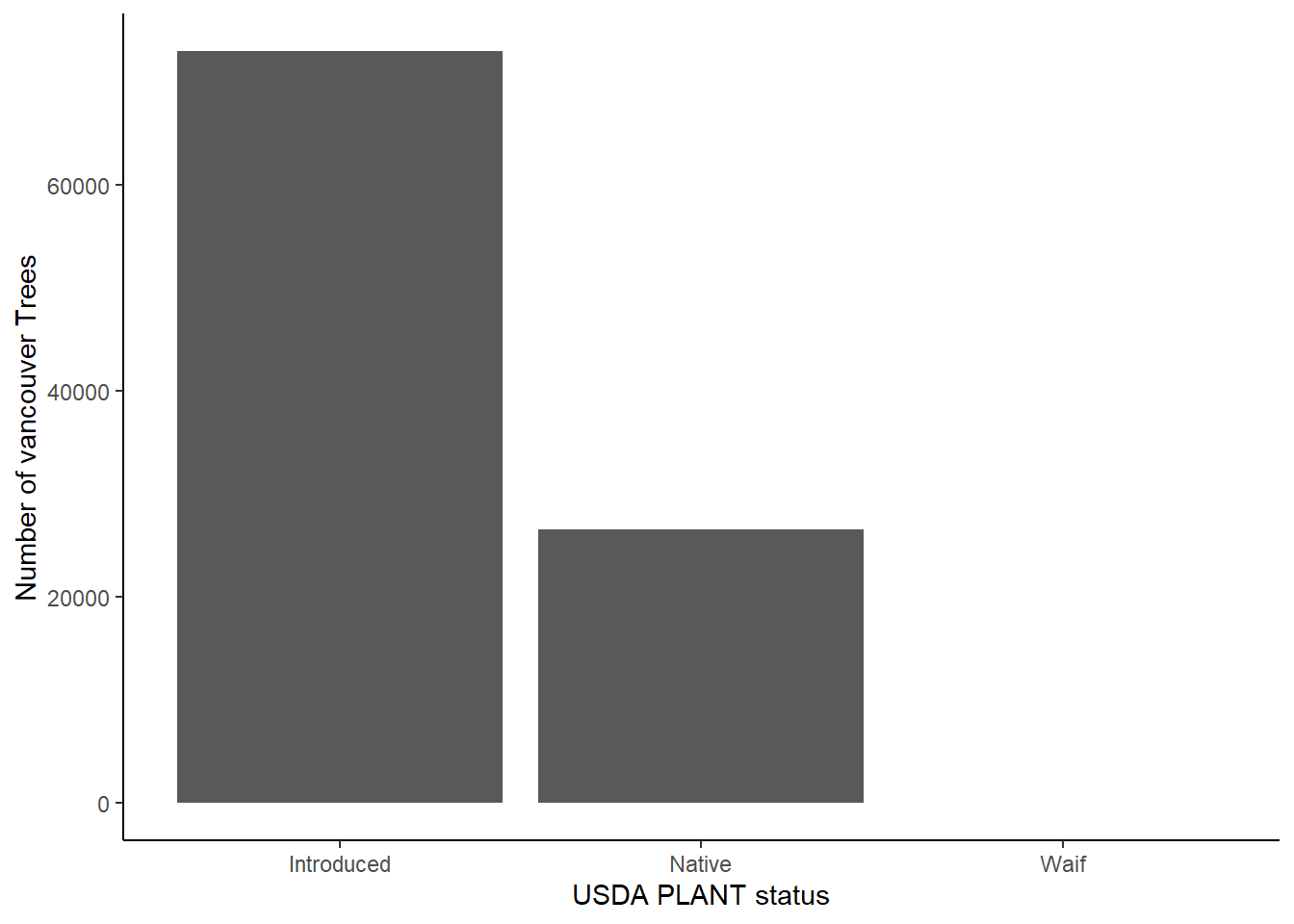
We can then visualize Vancouver for the number of trees.
library(viridis)## Loading required package: viridisLitespplot(raster_clip, "Number_of_trees", col.regions=c("grey10", viridis(64)), col="transparent")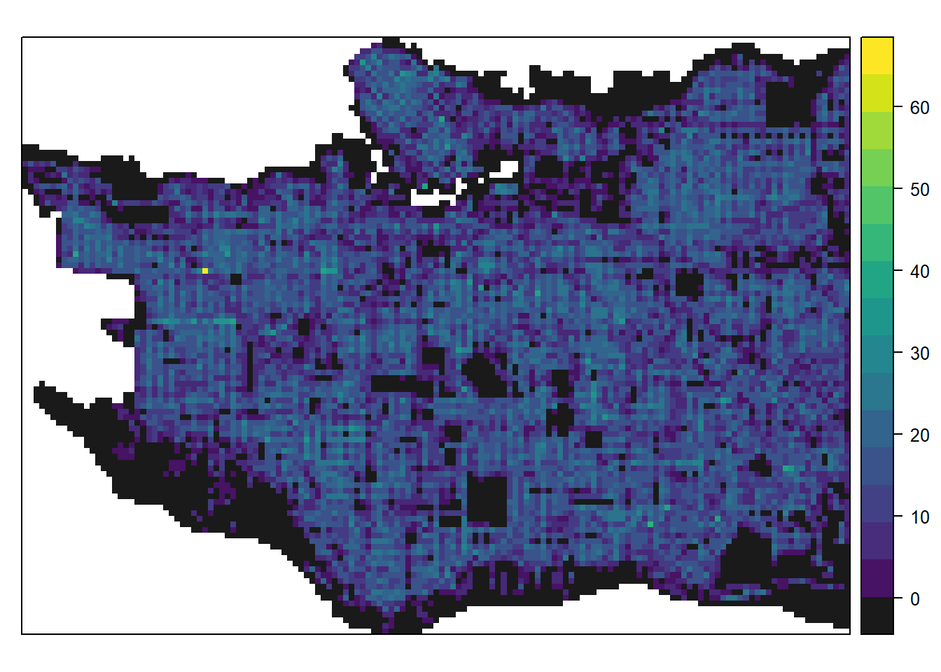
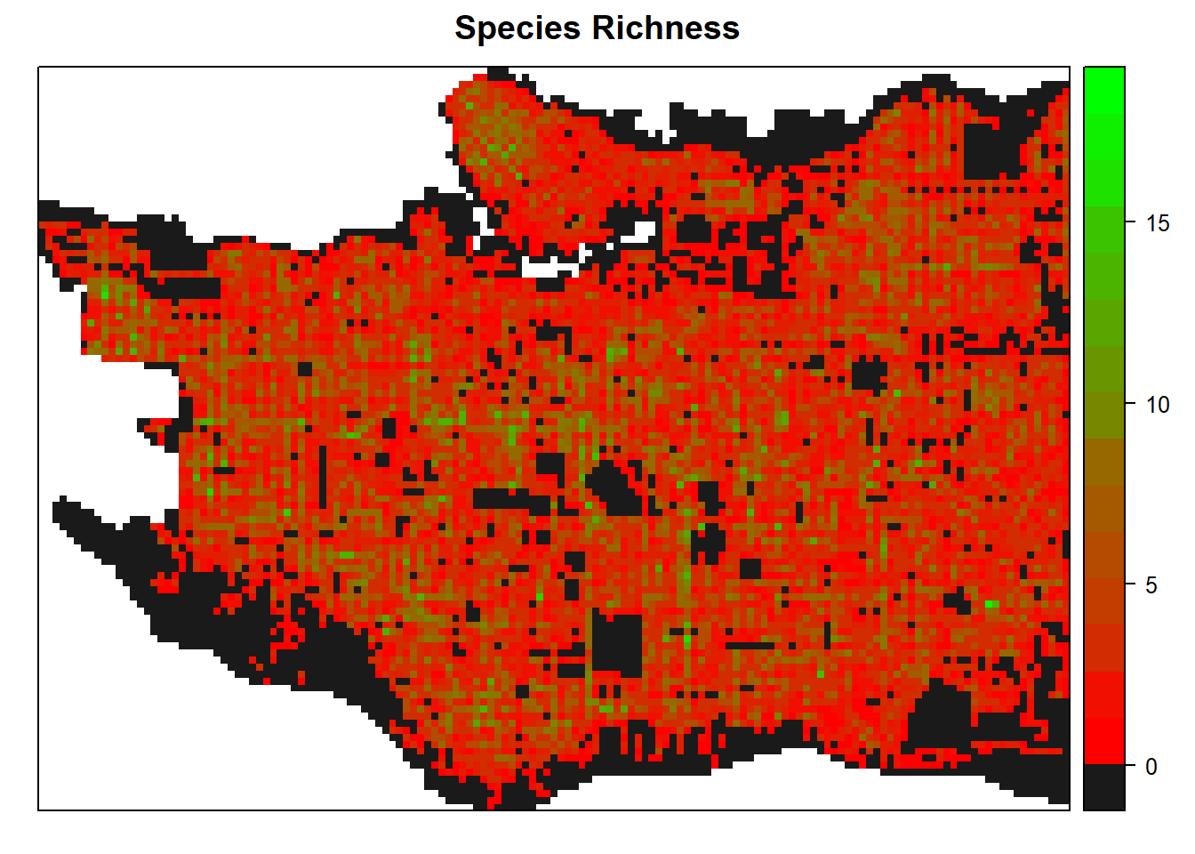
And species richness within each cell, this time using red to green scale from colorRamps.
spplot(raster_clip, "tree_richness", col.regions=c("grey10", rev(colorRamps::green2red(18))), col="transparent", main = "Species Richness")
And lastly, all cells with an introduced tree species.
spplot(raster_clip, "presence", col.regions=c("grey10", colorRamps::green2red(20)), col="transparent")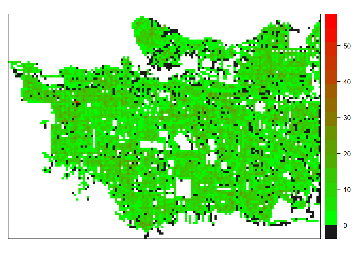
sessionInfo()## R version 3.6.1 (2019-07-05)
## Platform: x86_64-w64-mingw32/x64 (64-bit)
## Running under: Windows 10 x64 (build 18363)
##
## Matrix products: default
##
## locale:
## [1] LC_COLLATE=English_Canada.1252 LC_CTYPE=English_Canada.1252
## [3] LC_MONETARY=English_Canada.1252 LC_NUMERIC=C
## [5] LC_TIME=English_Canada.1252
##
## attached base packages:
## [1] stats graphics grDevices utils datasets methods base
##
## other attached packages:
## [1] viridis_0.5.1 viridisLite_0.3.0 ggplot2_3.2.1 vegan_2.5-6
## [5] lattice_0.20-38 permute_0.9-5 tidyr_1.0.2 purrr_0.3.3
## [9] rvest_0.3.5 xml2_1.2.2 httr_1.4.1 dplyr_0.8.4
## [13] raster_3.0-12 rgdal_1.4-8 sp_1.3-2
##
## loaded via a namespace (and not attached):
## [1] tidyselect_1.0.0 xfun_0.12 splines_3.6.1 colorspace_1.4-1
## [5] vctrs_0.2.2 htmltools_0.4.0 yaml_2.2.1 mgcv_1.8-28
## [9] rlang_0.4.4 pillar_1.4.3 glue_1.3.1 withr_2.1.2
## [13] lifecycle_0.1.0 stringr_1.4.0 rgeos_0.5-2 munsell_0.5.0
## [17] blogdown_0.17 gtable_0.3.0 codetools_0.2-16 evaluate_0.14
## [21] labeling_0.3 knitr_1.28 parallel_3.6.1 highr_0.8
## [25] Rcpp_1.0.3 scales_1.1.0 farver_2.0.3 gridExtra_2.3
## [29] digest_0.6.23 stringi_1.4.3 bookdown_0.17 grid_3.6.1
## [33] tools_3.6.1 magrittr_1.5 lazyeval_0.2.2 tibble_2.1.3
## [37] cluster_2.1.0 crayon_1.3.4 pkgconfig_2.0.3 MASS_7.3-51.4
## [41] Matrix_1.2-17 assertthat_0.2.1 rmarkdown_2.1 R6_2.4.1
## [45] colorRamps_2.3 nlme_3.1-144 compiler_3.6.1