Motivation: I created this image as part of a graduate course I audited in 2018. In short, I learned the very simple basics of working with a shapefile (.kml) in R. Otherwise, everything was done using ggplot2 and base R. It also was originally knit as an html file with tabs.
Data
City of Vancouver Trees dataset with locations (direct link download) City of Vancouver Neighbourhood Boundaries (direct link download)
Code
The first step is to download the two data files, one a text file containing tree locations, and the other a shapefile file containing polygons of Vancouver’s neighbourhoods, which outline the shape and geographical coordinates of each neighbourhood.
if (file.exists("StreetTrees_CityWide.csv")==F ) {
  download.file("ftp://webftp.vancouver.ca/OpenData/csv/csv_street_trees.zip", "csv_street_trees.zip")
  unzip(zipfile = "csv_street_trees.zip", files = "StreetTrees_CityWide.csv")
}

# download shapefile
if (file.exists("cov_localareas.kml")==F){
  download.file("http://data.vancouver.ca/download/kml/cov_localareas.kml", "cov_localareas.kml")
}
As the ZIP file of tree locations contain multiple csv files for each neighbourhood as well as the entire city, we extracted only the file with all the trees.
To examine the contents of a zip file in R, use the list argument to list files:
unzip(zipfile = "path_to_zip_file", list=T)This will list the files in the zip archive rather than extract all. unzip("path_to_zip_file") will extract the entire zip archive.
To read in the data files, I used rgdal to read in the KML file.
# install.packages("rgdal")
library(rgdal)
## Warning: package 'rgdal' was built under R version 3.6.2## Loading required package: sp## Warning: package 'sp' was built under R version 3.6.2## rgdal: version: 1.4-8, (SVN revision 845)
## Geospatial Data Abstraction Library extensions to R successfully loaded
## Loaded GDAL runtime: GDAL 2.2.3, released 2017/11/20
## Path to GDAL shared files: C:/Users/YIHANWU/Documents/R/win-library/3.6/rgdal/gdal
## GDAL binary built with GEOS: TRUE
## Loaded PROJ.4 runtime: Rel. 4.9.3, 15 August 2016, [PJ_VERSION: 493]
## Path to PROJ.4 shared files: C:/Users/YIHANWU/Documents/R/win-library/3.6/rgdal/proj
## Linking to sp version: 1.3-2locmap<-readOGR("cov_localareas.kml", "local_areas_region", stringsAsFactors = F)## OGR data source with driver: KML
## Source: "C:\Users\YIHANWU\Documents\Stuff\blogdown-ywu\content\post\cov_localareas.kml", layer: "local_areas_region"
## with 22 features
## It has 2 fieldsReading in the trees file is simple with read.csv() or you can use readr::read._csv() if you have the readr installed.
treedat<-read.csv("StreetTrees_CityWide.csv")
summary(treedat)
## TREE_ID CIVIC_NUMBER STD_STREET
## Min. : 12 Min. : 0 CAMBIE ST : 1651
## 1st Qu.: 63434 1st Qu.: 1306 W KING EDWARD AV: 1616
## Median :130873 Median : 2607 W 13TH AV : 1251
## Mean :128158 Mean : 2942 W 16TH AV : 1155
## 3rd Qu.:190392 3rd Qu.: 4012 W 14TH AV : 1116
## Max. :259643 Max. :17888 W 15TH AV : 1087
## (Other) :137190
## NEIGHBOURHOOD_NAME ON_STREET ON_STREET_BLOCK
## RENFREW-COLLINGWOOD :11313 CAMBIE ST : 1590 Min. : 0
## KENSINGTON-CEDAR COTTAGE:11264 W KING EDWARD AV: 1507 1st Qu.:1300
## HASTINGS-SUNRISE :10254 W 16TH AV : 1111 Median :2600
## DUNBAR-SOUTHLANDS : 9334 W 13TH AV : 1081 Mean :2912
## SUNSET : 8355 W 37TH AV : 967 3rd Qu.:4000
## KITSILANO : 8010 W 15TH AV : 949 Max. :9900
## (Other) :86536 (Other) :137861
## STREET_SIDE_NAME ASSIGNED HEIGHT_RANGE_ID DIAMETER
## BIKE MED: 38 N:129569 Min. : 0.000 Min. : 0.00
## EVEN :70915 Y: 15497 1st Qu.: 1.000 1st Qu.: 3.00
## MED : 3293 Median : 2.000 Median : 8.50
## ODD :70685 Mean : 2.621 Mean : 11.25
## PARK : 68 3rd Qu.: 3.000 3rd Qu.: 16.00
## TBD : 67 Max. :10.000 Max. :1819.00
##
## DATE_PLANTED PLANT_AREA ROOT_BARRIER CURB
## Min. :19891027 10 :20438 N:135803 N: 12736
## 1st Qu.:20040225 8 :15651 Y: 9263 Y:132330
## Median :20180128 N :13944
## Mean :20112434 6 :13813
## 3rd Qu.:20180128 7 :11857
## Max. :20180128 12 : 9210
## (Other):60153
## CULTIVAR_NAME GENUS_NAME SPECIES_NAME
## :67157 ACER :35551 SERRULATA :13513
## KWANZAN :10658 PRUNUS :31134 CERASIFERA :12455
## ATROPURPUREUM: 9340 FRAXINUS: 7332 PLATANOIDES:12008
## FASTIGIATA : 4119 TILIA : 6884 RUBRUM : 8292
## NIGRA : 3261 QUERCUS : 5981 AMERICANA : 5562
## BOWHALL : 2455 CARPINUS: 5679 BETULUS : 5116
## (Other) :48076 (Other) :52505 (Other) :88120
## COMMON_NAME LATITUDE LONGITUDE
## KWANZAN FLOWERING CHERRY : 10658 Min. : 0.00 Min. :-123.2
## PISSARD PLUM : 9103 1st Qu.:49.22 1st Qu.:-123.1
## NORWAY MAPLE : 5683 Median :49.24 Median :-123.1
## CRIMEAN LINDEN : 4489 Mean :42.21 Mean :-105.5
## PYRAMIDAL EUROPEAN HORNBEAM: 3446 3rd Qu.:49.26 3rd Qu.:-123.0
## NIGHT PURPLE LEAF PLUM : 3261 Max. :49.29 Max. : 0.0
## (Other) :108426The tree dataframe contains 20 column which thankfully come with self-explanatory column names. Weirdly enough, everything is in capitals.
head(treedat)## TREE_ID CIVIC_NUMBER STD_STREET NEIGHBOURHOOD_NAME ON_STREET
## 1 589 4694 W 8TH AV WEST POINT GREY BLANCA ST
## 2 592 1799 W KING EDWARD AV SHAUGHNESSY W KING EDWARD AV
## 3 594 2401 W 1ST AV KITSILANO W 1ST AV
## 4 595 2405 W 1ST AV KITSILANO W 1ST AV
## 5 596 2428 W 1ST AV KITSILANO W 1ST AV
## 6 598 2428 W 1ST AV KITSILANO W 1ST AV
## ON_STREET_BLOCK STREET_SIDE_NAME ASSIGNED HEIGHT_RANGE_ID DIAMETER
## 1 2400 EVEN N 5 32
## 2 1700 MED N 1 3
## 3 2400 ODD N 4 14
## 4 2400 ODD N 2 3
## 5 2400 EVEN N 2 11
## 6 2400 EVEN N 2 3
## DATE_PLANTED PLANT_AREA ROOT_BARRIER CURB CULTIVAR_NAME GENUS_NAME
## 1 20180128 B N Y ALNUS
## 2 20100104 30 N Y ABIES
## 3 20180128 B N Y PINUS
## 4 19970109 B N Y CALOCARPA MALUS
## 5 20180128 B N Y PRUNUS
## 6 20180128 B N Y PRUNUS
## SPECIES_NAME COMMON_NAME LATITUDE LONGITUDE
## 1 RUGOSA SPECKLED ALDER 49.26532 -123.2150
## 2 GRANDIS GRAND FIR 49.24952 -123.1457
## 3 NIGRA AUSTRIAN PINE 49.27096 -123.1599
## 4 ZUMI REDBUD CRABAPPLE 0.00000 0.0000
## 5 SARGENTII SARGENT FLOWERING CHERRY 49.27083 -123.1602
## 6 SARGENTII SARGENT FLOWERING CHERRY 49.27084 -123.1605We can drop those columns which we don’t need.
treedat <- treedat[, c("COMMON_NAME", "LATITUDE", "LONGITUDE")]To map cherry trees across Vancouver, we first have to filter out the cherry trees. As treedat has a COMMON_NAME column, a string match using grep on that column will tell us which trees have “cherry” in their name and we can subset the entire dataframe for only cherry trees.
cherry_trees<-treedat[grep("cherry", treedat$COMMON_NAME, ignore.case = T),]By using ignore.case = T, we do case-insensitive pattern matching without the need to specify “CHERRY” in the pattern argument.
dim(cherry_trees)## [1] 18245 3There are nrow(cherry_trees) in Vancouver. We could just plot all of them and be done, but since we have cultivar information, we can examine individual cultivar distribution across the city. First, we use a table to get the different cherries by cultivars, and how many there are.
cherry_names<-as.data.frame(table(cherry_trees$COMMON_NAME))Then we sort the table by the most frequent cultivars.
top_cherry_names<-cherry_names[order(-cherry_names$Freq),]
head(top_cherry_names, n = 10)
## Var1 Freq
## 303 KWANZAN FLOWERING CHERRY 10658
## 2 AKEBONO FLOWERING CHERRY 2295
## 554 UKON JAPANESE CHERRY 856
## 346 MAZZARD CHERRY 603
## 402 PINK PERFECTION CHERRY 529
## 435 RANCHO SARGENT CHERRY 513
## 280 JAPANESE FLOWERING CHERRY 484
## 482 SHIROFUGEN CHERRY 340
## 483 SHIROTAE(MT FUJI) CHERRY 229
## 472 SCHUBERT CHOKECHERRY 214Kwanzan Flowering Cherry appears to be the most common. I will take only the top nine cultivars, and then filter my cherry tree dataset for only the trees with common names matching one of the top nine.
top_cultivars<-top_cherry_names[1:9,]
cherry_filtered<-cherry_trees[cherry_trees$COMMON_NAME %in% top_cultivars$Var1,]
summary(cherry_filtered)
## COMMON_NAME LATITUDE LONGITUDE
## KWANZAN FLOWERING CHERRY:10658 Min. : 0.00 Min. :-123.2
## AKEBONO FLOWERING CHERRY: 2295 1st Qu.:49.22 1st Qu.:-123.1
## UKON JAPANESE CHERRY : 856 Median :49.24 Median :-123.1
## MAZZARD CHERRY : 603 Mean :43.65 Mean :-109.1
## PINK PERFECTION CHERRY : 529 3rd Qu.:49.26 3rd Qu.:-123.1
## RANCHO SARGENT CHERRY : 513 Max. :49.29 Max. : 0.0
## (Other) : 1053But some trees seem to have wonky latitude or longitude coordinates. If we look at the distribution, these values stand part from the group
hist(cherry_filtered$LATITUDE)
hist(cherry_filtered$LONGITUDE)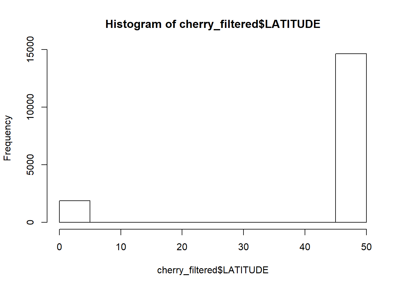
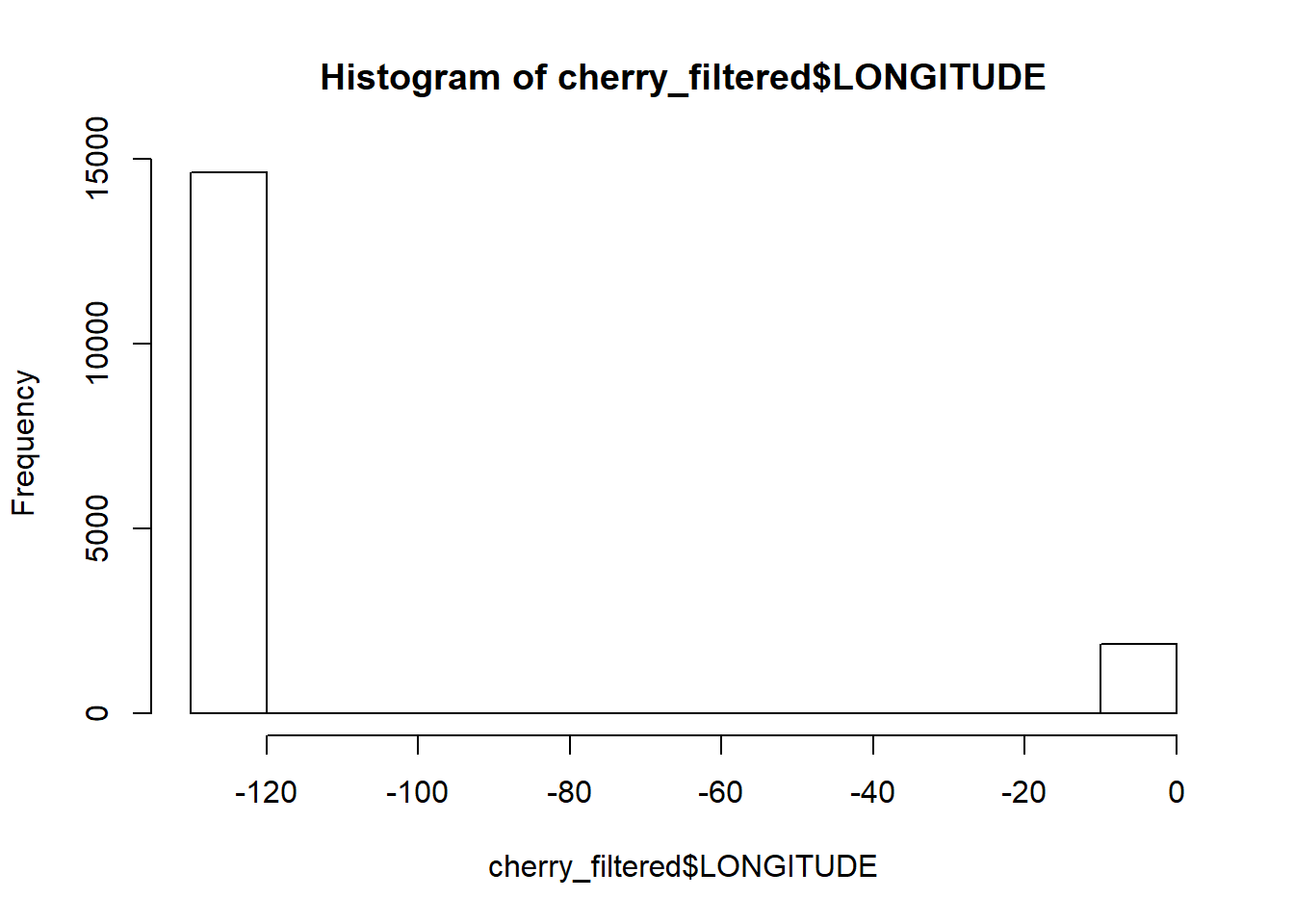
We can get rid of them by roughly excluding them through subsetting based on value. All trees must have a latitude value greater than 40 and a longitude smaller than -100.
cherry_filtered<-cherry_filtered[cherry_filtered$LATITUDE > 40 & cherry_filtered$LONGITUDE < -100,]I don’t like the fact everything is in capitals but R (and its help pages) are always there to save the day. Making everything lowercase is through tolower(), and its opposite is the toupper() function. But for sentence case, the simpleCap function is from the examples is the easiest solution. There is also a more complicated capwords function but simpleCap works well enough.
simpleCap <- function(x) {
  s <- strsplit(x, " ")[[1]]
  paste(toupper(substring(s, 1,1)), substring(s, 2),
        sep="", collapse=" ")
}
What simpleCap does is takes in a string such as “the quick red fox jumps over the lazy brown dog”, splits each word into letters, and then capitalizes the first letter before pasting all the letters in the word back together.
For example,
simpleCap("the quick red fox jumps over the lazy brown dog")## [1] "The Quick Red Fox Jumps Over The Lazy Brown Dog"We can use the sapply() function to use this simpleCap function on every row of the COMMON_NAME column.
cherry_filtered$COMMON_NAME<-sapply(as.character(tolower(cherry_filtered$COMMON_NAME)), simpleCap)
head(cherry_filtered)
## COMMON_NAME LATITUDE LONGITUDE
## 8 Kwanzan Flowering Cherry 49.27096 -123.1601
## 12 Kwanzan Flowering Cherry 49.27097 -123.1605
## 24 Kwanzan Flowering Cherry 49.27086 -123.1615
## 25 Kwanzan Flowering Cherry 49.27086 -123.1615
## 71 Shirotae(mt Fuji) Cherry 49.27062 -123.1466
## 72 Shirotae(mt Fuji) Cherry 49.27062 -123.1467Notice that the capitalization for Shirotae did not work inside the parantheses due to the lack of a space making it a separate word.
simpleCap("Shirotae(mt Fuji)")## [1] "Shirotae(mt Fuji)"But if we manually add a space, it still does not work.
simpleCap("Shirotae (mt Fuji)")## [1] "Shirotae (mt Fuji)"But rather, this is because the ( character is the first letter rather than m.
simpleCap("Shirotae ( mt Fuji)")## [1] "Shirotae ( Mt Fuji)"In this case, we can just manually correct this error by editing every “Shirotae(mt Fuji)” string.
We first make the cultivar names into factors, and then edit the level name with the corrected capitalization.
str(cherry_filtered)## 'data.frame': 14631 obs. of 3 variables:
## $ COMMON_NAME: chr "Kwanzan Flowering Cherry" "Kwanzan Flowering Cherry" "Kwanzan Flowering Cherry" "Kwanzan Flowering Cherry" ...
## $ LATITUDE : num 49.3 49.3 49.3 49.3 49.3 ...
## $ LONGITUDE : num -123 -123 -123 -123 -123 ...cherry_filtered$COMMON_NAME<-as.factor(cherry_filtered$COMMON_NAME)
str(cherry_filtered)## 'data.frame': 14631 obs. of 3 variables:
## $ COMMON_NAME: Factor w/ 9 levels "Akebono Flowering Cherry",..: 3 3 3 3 8 8 8 8 3 3 ...
## $ LATITUDE : num 49.3 49.3 49.3 49.3 49.3 ...
## $ LONGITUDE : num -123 -123 -123 -123 -123 ...levels(cherry_filtered$COMMON_NAME)[levels(cherry_filtered$COMMON_NAME)=="Shirotae(mt Fuji) Cherry"] <- "Shirotae (Mt Fuji) Cherry"
head(cherry_filtered)## COMMON_NAME LATITUDE LONGITUDE
## 8 Kwanzan Flowering Cherry 49.27096 -123.1601
## 12 Kwanzan Flowering Cherry 49.27097 -123.1605
## 24 Kwanzan Flowering Cherry 49.27086 -123.1615
## 25 Kwanzan Flowering Cherry 49.27086 -123.1615
## 71 Shirotae (Mt Fuji) Cherry 49.27062 -123.1466
## 72 Shirotae (Mt Fuji) Cherry 49.27062 -123.1467Onto the plot!
ggplot2 does not accept spatial objects such as a SpatialPolygonsDataFrame directly so we have to modify it into a dataframe. Spatial packages in R have their own plotting methods to plot spatial objects.
library(ggplot2)
vancouver_map<-fortify(locmap, region="Name")
head(vancouver_map)
## long lat order hole piece id group
## 1 -123.1641 49.25748 1 FALSE 1 Arbutus-Ridge Arbutus-Ridge.1
## 2 -123.1639 49.25746 2 FALSE 1 Arbutus-Ridge Arbutus-Ridge.1
## 3 -123.1636 49.25745 3 FALSE 1 Arbutus-Ridge Arbutus-Ridge.1
## 4 -123.1626 49.25743 4 FALSE 1 Arbutus-Ridge Arbutus-Ridge.1
## 5 -123.1603 49.25740 5 FALSE 1 Arbutus-Ridge Arbutus-Ridge.1
## 6 -123.1579 49.25736 6 FALSE 1 Arbutus-Ridge Arbutus-Ridge.1Here, you can see the latitudes and longitude of each point, the order each point is plotted in with lines that will connect the points, and also columns designating which groups the points belong to.
The first thing to plot is our neighbourhoods. Don’t forget by convention longitude is usually plotted on the x-axis and latitude on the y.
p <- ggplot(data=vancouver_map, aes(x=long, y=lat)) +
  geom_path(aes(group=group))
p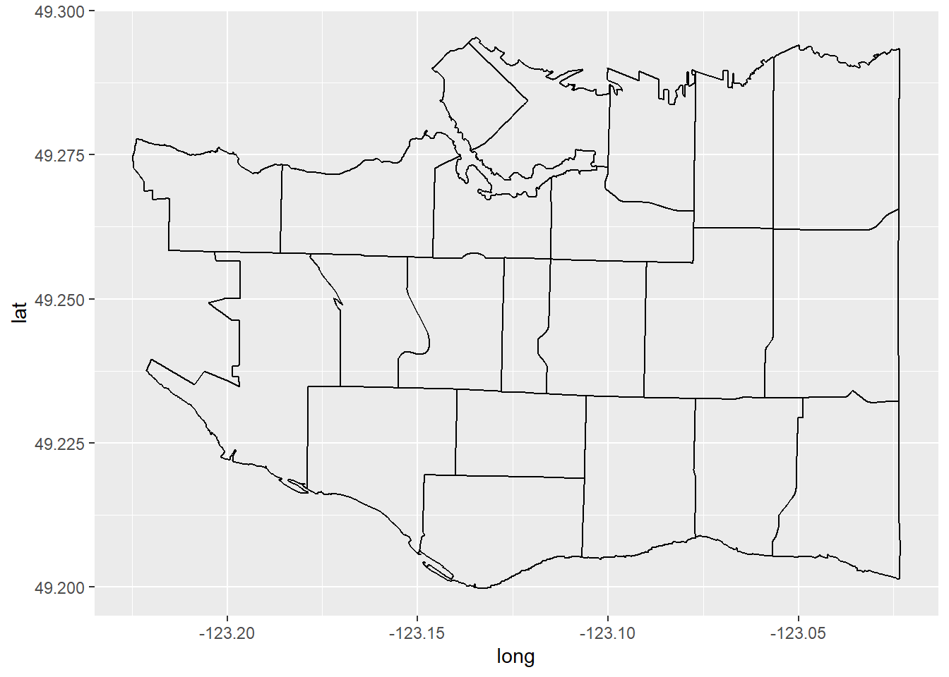
We can use a different theme to get rid of the grey background.
p <- p + theme_void()
p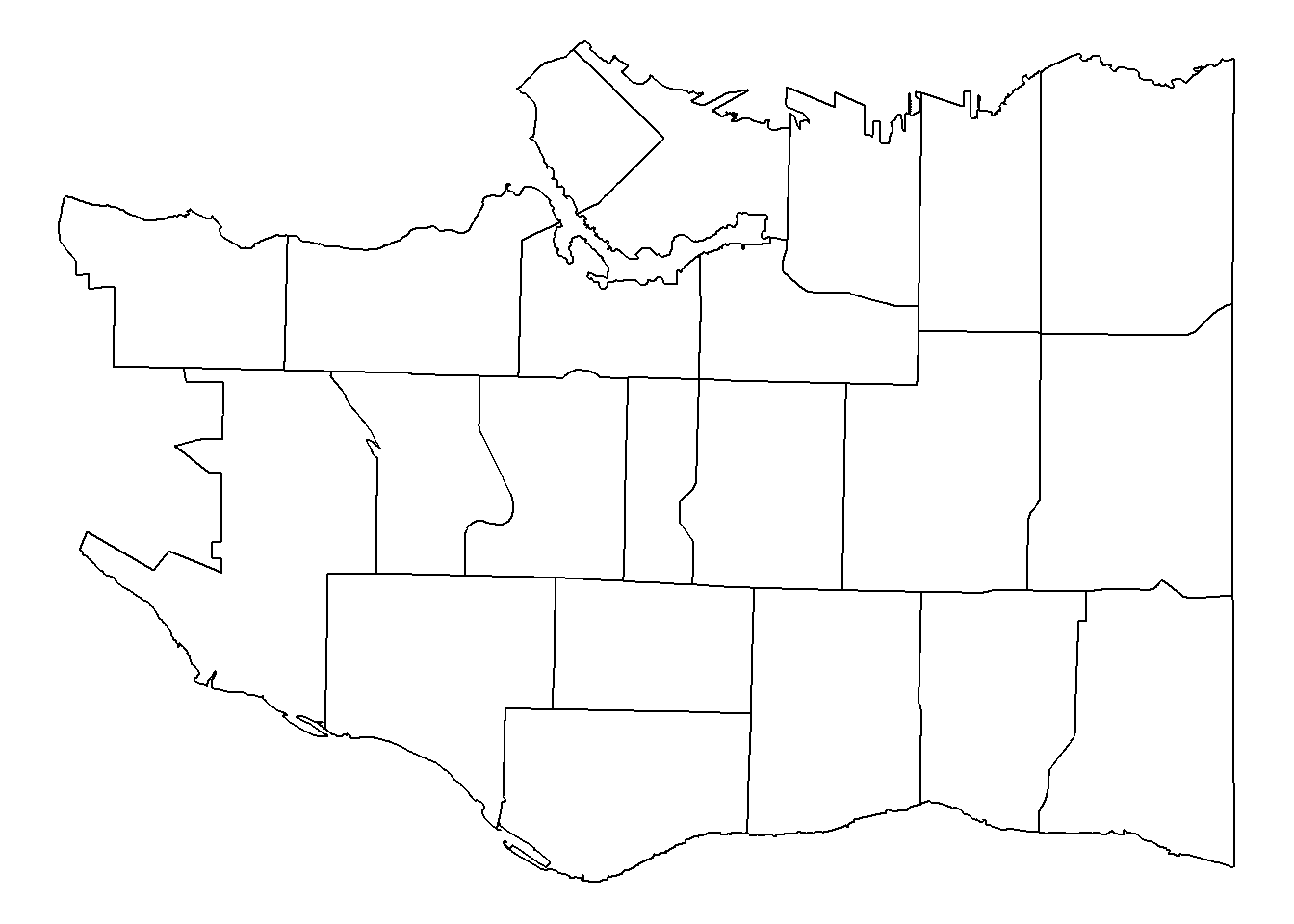
We can plot each tree as a single point.
p + geom_point(data = cherry_filtered, aes(x=LONGITUDE, y=LATITUDE))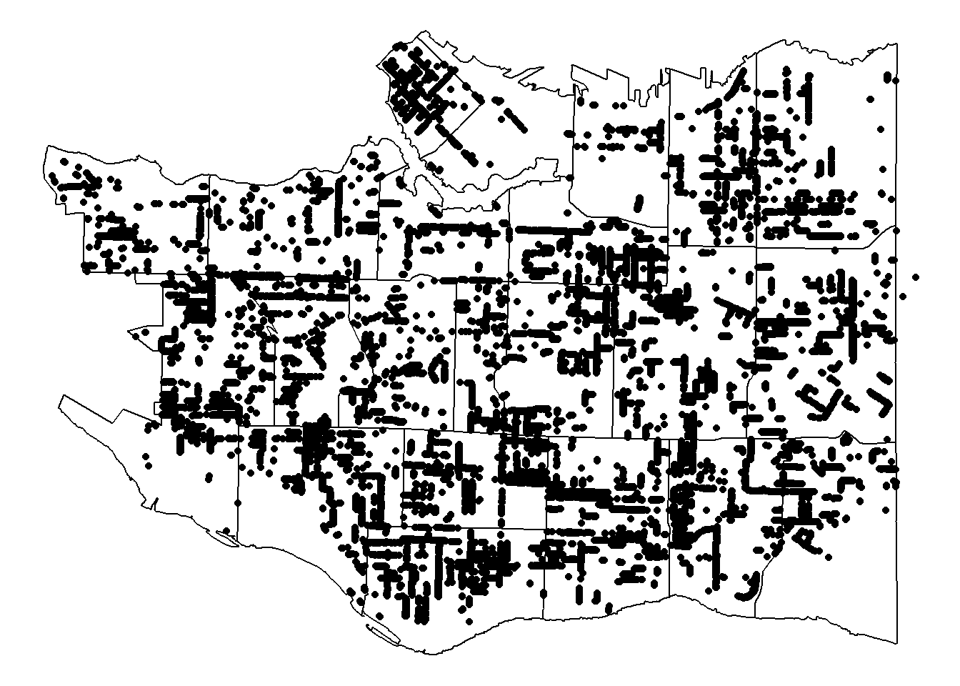
You can see the points outlining the streets and overplotting in dense areas. We can use a density geom instead by dividing the plot up into smaller areas and counting up the number of trees in them.
p + stat_bin2d(data = cherry_filtered, aes(x=LONGITUDE, y=LATITUDE))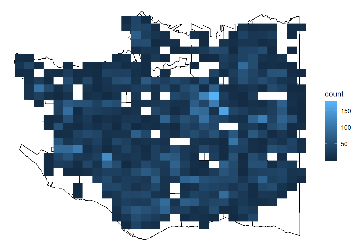
Using more bins … …
q <- p + stat_bin2d(data = cherry_filtered, aes(x=LONGITUDE, y=LATITUDE), bins=40)

q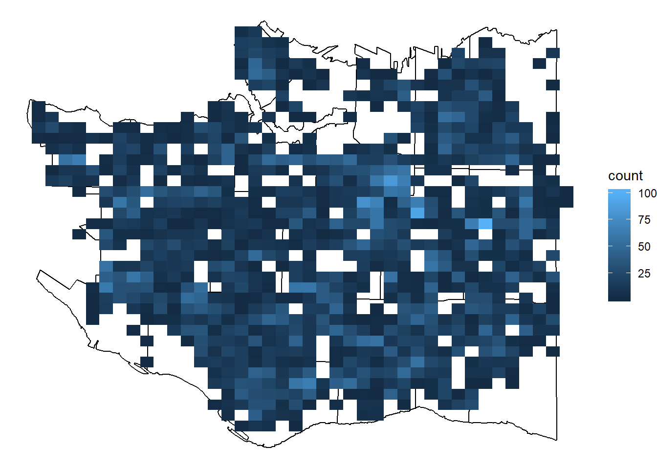
We can facet the plot for the nine different cultivars in a 3 by 3 grid. And add a caption for the data source as well as a figure title.
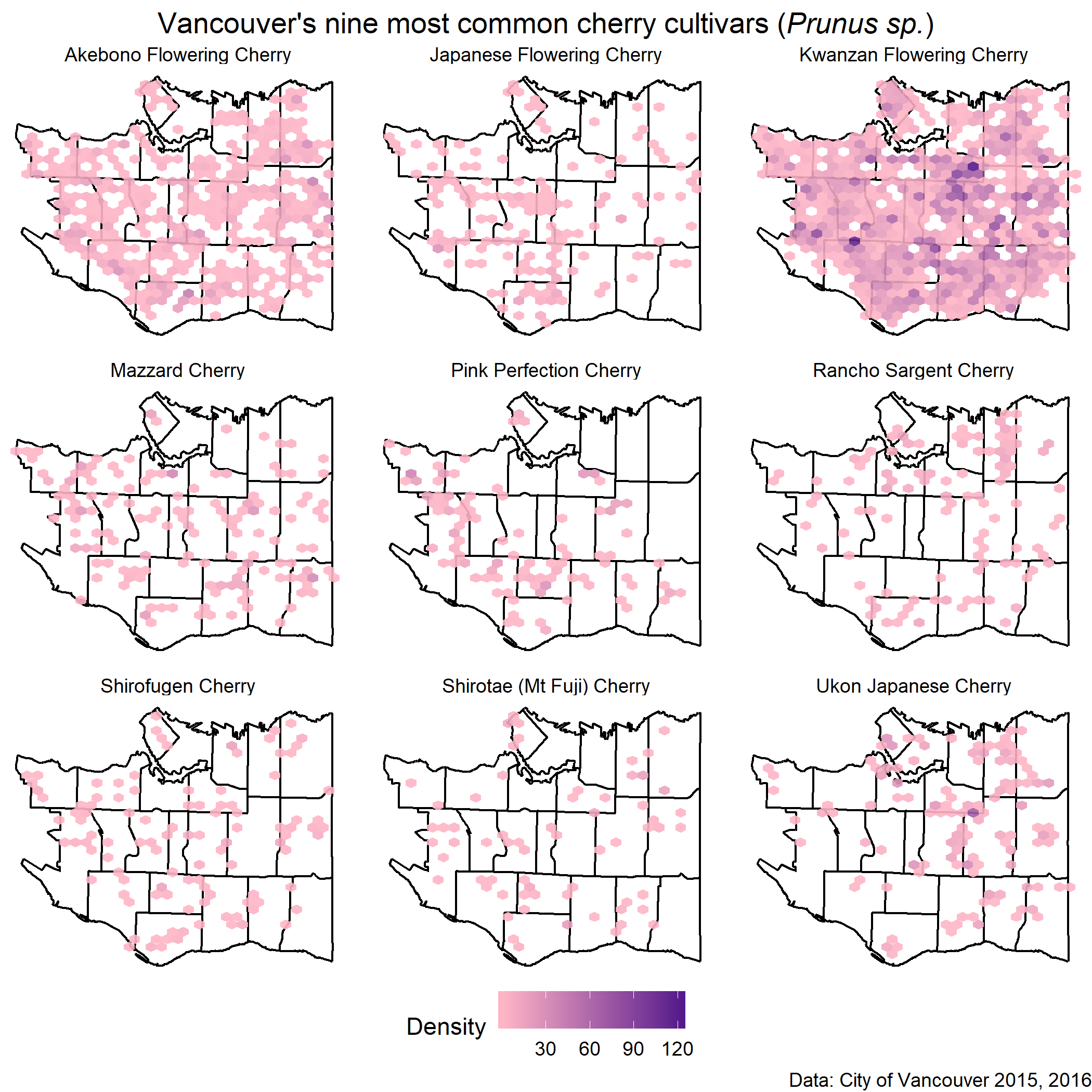
figure_title<-expression(paste("Vancouver's nine most common cherry cultivars (", italic("Prunus sp."), ")"))

q <- q + facet_wrap(~COMMON_NAME, nrow=3) + labs(x=NULL, y=NULL, title=figure_title, caption="Data: City of Vancouver 2015, 2016")
q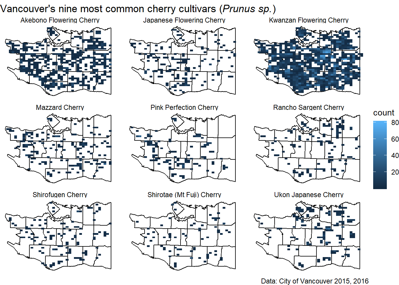
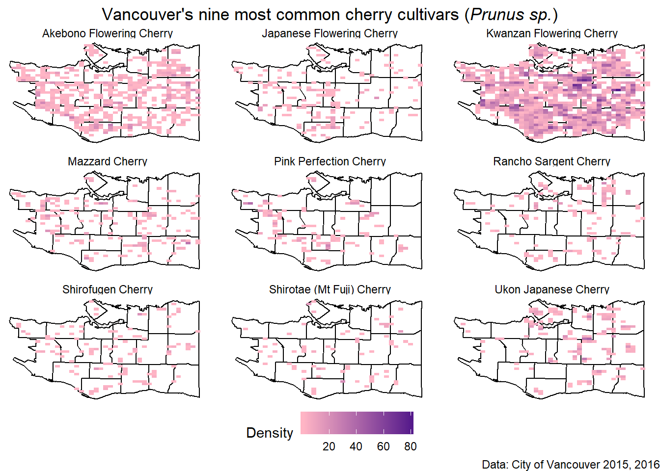
To fit with the cherries, we can modify the colors used. It’s also possible to move the legend to the bottom and make it a horizontal scale.
q +
  scale_fill_gradient(low="pink1", high="purple4", name="Density") +
  theme(legend.direction = "horizontal",
        legend.position = "bottom",
        plot.title = element_text(hjust=0.5)
) 
Lastly, rather than use square, it is possible to use hexagonal bins.
cherrymap<-ggplot(data=vancouver_map, aes(x=long, y=lat)) +
  geom_path(aes(group=group))+
  geom_hex(data=cherry_filtered, aes(x=LONGITUDE, y=LATITUDE), alpha=0.9, bins=30) +
  scale_fill_gradient(low="pink1", high="purple4", name="Density") +
  theme_void() + facet_wrap(~COMMON_NAME, nrow=3) +
  labs(x=NULL, y=NULL, title=figure_title, caption="Data: City of Vancouver 2015, 2016") +
  theme(legend.direction = "horizontal",
        legend.position = "bottom",
        plot.title = element_text(hjust=0.5)
        )
Final Product
cherrymap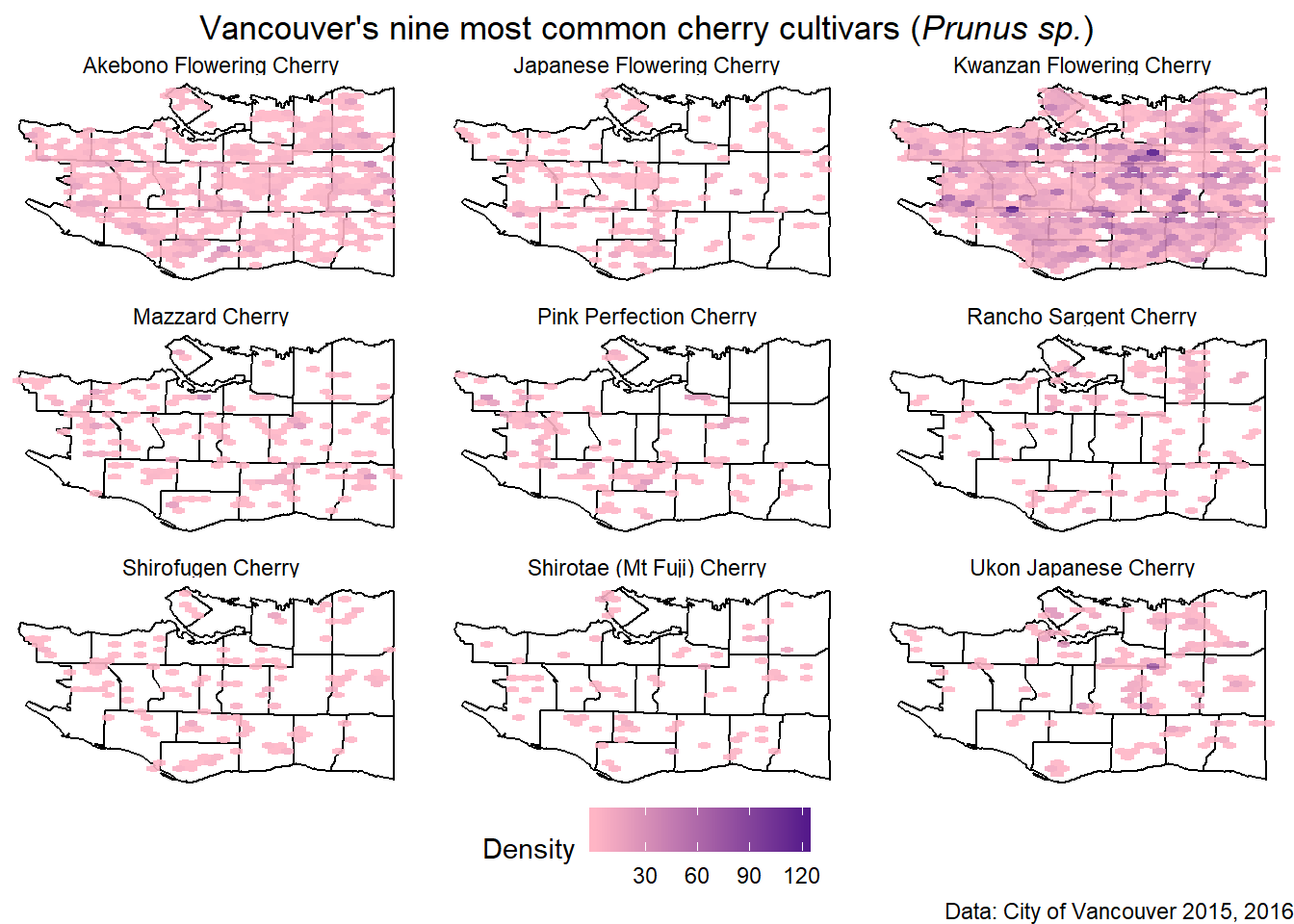
And all the cherry trees plotted together.
all_cherry <- ggplot(data=vancouver_map, aes(x=long, y=lat)) +
  geom_path(aes(group=group))+
  geom_hex(data=cherry_filtered, aes(x=LONGITUDE, y=LATITUDE), alpha=0.9, bins=60) +
  scale_fill_gradient(low="pink1", high="purple4", name="Density") +
  theme_void() +
  labs(x=NULL, y=NULL, title="Vancouver's Cherry Trees", caption="Data: City of Vancouver 2015, 2016") +
  theme(legend.direction = "horizontal",
        legend.position = "bottom",
        plot.title = element_text(hjust=0.5)
        )
all_cherry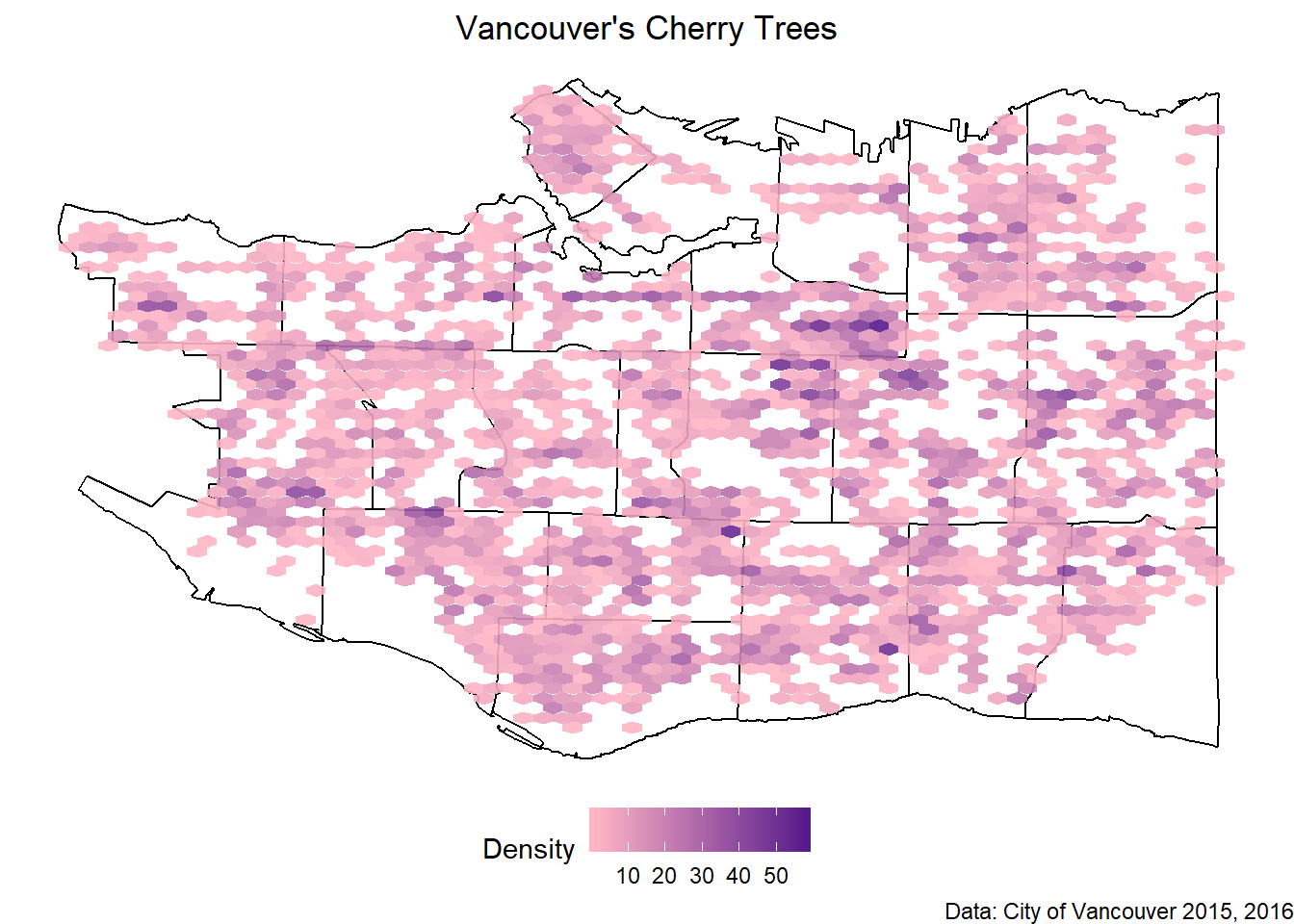
And the names of the neighbourhoods.
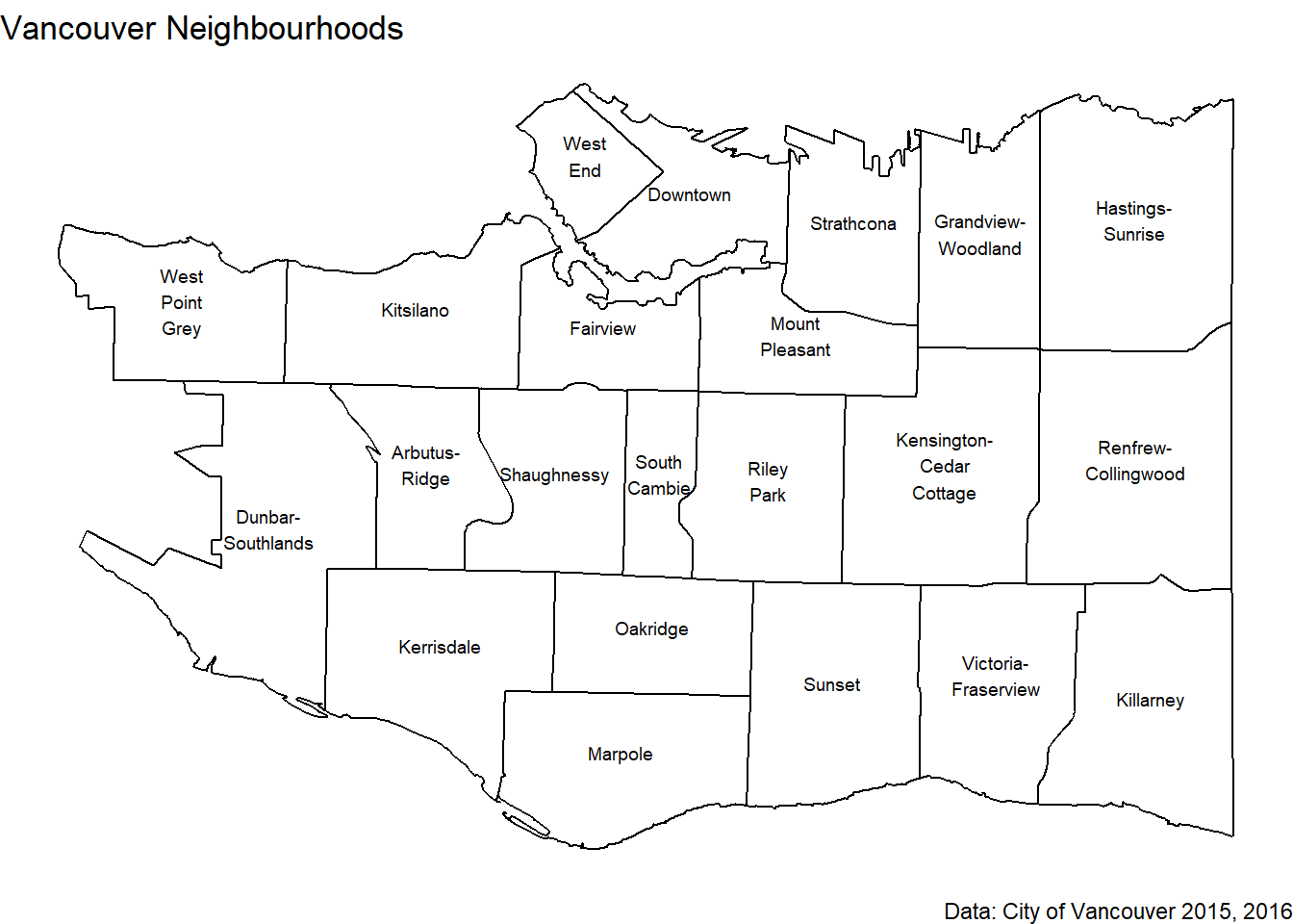
In conclusion, go to Mount Pleasant for the most cherry trees!