Parameter testing In stacks, SNP extraction and visualization in R

The recommended way to figure out the best parameters to use in stacks for denovo RAD-seq analysis is to test parameter combinations for M and n. (Paris et al. 2017, Rochette and Catchen 2017).

The authors of stacks recommend testing M and n from 1 to 9 and then visualizing the distribution of loci against the number of SNPs on the loci.

From Rochette and Catchen 2017

stacks provides a script to extract distributions using stacks-dist-extract but you will have to run it repeatedly by hand for every parameter.

Here is a bash script with a loop to extract the distribution of SNPs for each parameter combination and a R script to visualize the distributions in R similar to Rocheete and Catchen’s figure.

In this script, it is assumed that folder names follow Rochette and Catchen’s protocol (stacks.M1, stacks.M2 etc)

Home
+-- stacks.M1
|   +-- populations.r80
|   +-- populations.log
|   +-- populations.log.distribs
|   +-- ind.1.alleles.tsv.gz
|   +-- ind.1.matches.bam
|   +-- ind.1.snps.tsv.gz
|   +-- ind.1.tags.tsv.gz 
|   ...
|-- stacks.M2
|-- stacks.M3
|-- stacks.M4
...

#!/bin/bash

# load stacks for those who are on clusters, this is for SLURM
module load stacks/2.0b
# change the numbers in the next line to match the directory values
for i in 1 2 3 4 5 6 7 8 9
do
  stacks-dist-extract stacks.M${i}/populations.r80/populations.log.distribs snps_per_loc_postfilters > ${i}_snp_distribution.tsv
done

There is also a pure awk solution not involving stacks scripts.

#!/bin/bash

# load stacks for those who are on clusters, this is for SLURM
module load stacks/2.0b

for i in 1 2 3 4 5 6 7 8 9
do
        awk '/snps_per_loc_postfilters/{flag=1; next} /END/{flag=0} flag' stacks.M${i}/populations.r80/populations.log.distribs > ${i}_snp_distribution.tsv
done

Then in R, make a data frame combining all parameter distributions before visualizaing in ggplot2. Here, the data comes from a GBS analysis of garlic mustard (Alliaria petiolata).

count <- 1
files <- list.files(path = "", pattern="*_snp_distribution.tsv", full.names = T)
for (i in files[1:9]){
  table <- read.delim(i, skip=1, header=T)
  table$n_loci_percent<- table$n_loci/sum(table$n_loci)
  table$m<- count
  write.table(table, "distributions.tsv", append=T, row.names=F, col.names = F)
  snp_count <- data.frame("m"= count, "n_snps"=sum(table$n_loci))
  write.table(snp_count, "total_count.tsv", append=T, row.names=F, col.names = F)
  count <- count + 1
}

total_count.tsv is used to display total SNP by parameter.

library(ggplot2)
snp_count<-read.delim("total_count.tsv", sep=" ", header=F)
names(snp_count)<-c("m", "n_snps")
snp_count$m<-as.factor(snp_count$m)
p<-ggplot(data=snp_count, aes(x=m, y=n_snps)) +
  geom_point() + theme_classic() + scale_y_continuous(limits = c(0, 3000))
p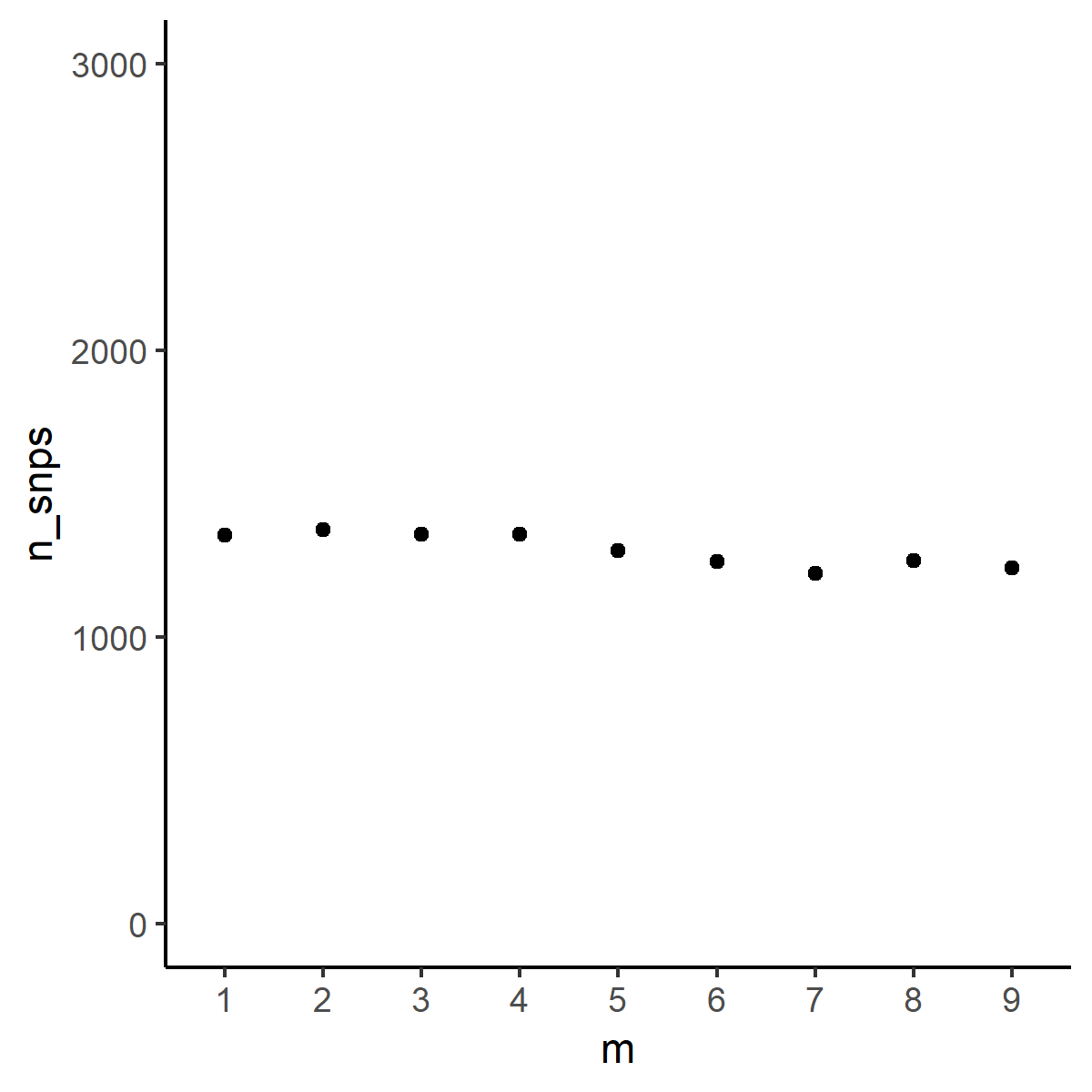

Scatterplot of parameter and total SNP count

distributions.tsv is used to show parameter distributions.

snp_table<-read.delim("distributions.tsv", sep=" ", header=F)
names(snp_table)<- c("n_snps","n_loci", "n_loci_percent", "m") 
snp_table$n_loci_percent<-snp_table$n_loci_percent*100
snp_table$n_snps<-ifelse(snp_table$n_snps < 9, snp_table$n_snps, "9 +")
snp_table$n_snps<-as.factor(snp_table$n_snps)
snp_table$m<-as.factor(snp_table$m)

q<-ggplot(data = snp_table) + 
  geom_col(aes(x=n_snps, y=n_loci_percent, fill=m), position="dodge") + theme_classic()
q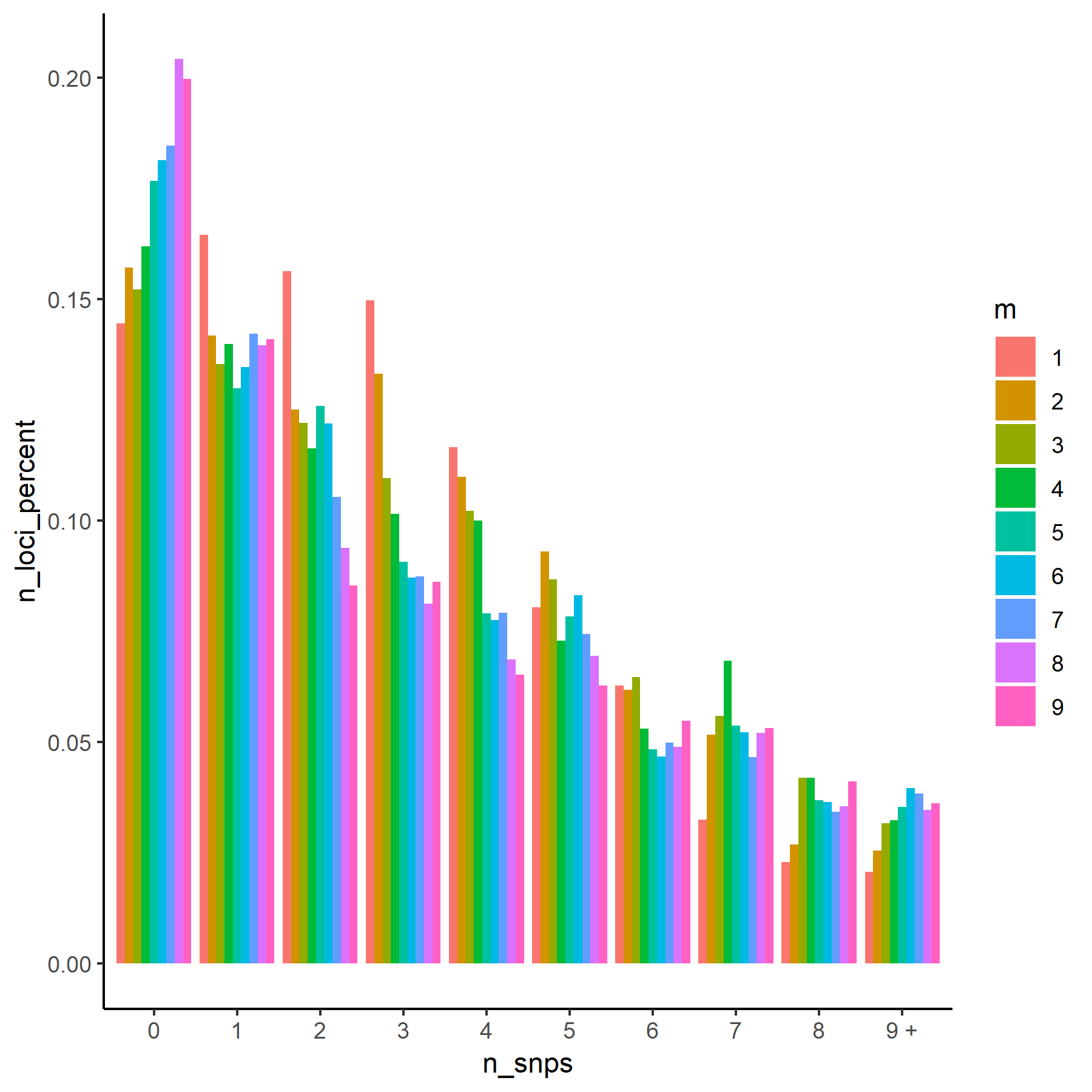

Histogram of number of SNPs per locus